csv2graph Sample Gallery
This gallery lets you explore the main csv2graph options with real sample data. Reproduce the sample directory layout shown in each section and you can run the commands exactly as written.
Every sample's CSV file is available for direct download on this page. Pre-rendered images and helper scripts are included when they add context.
Sample 1: Basic Overlay Only
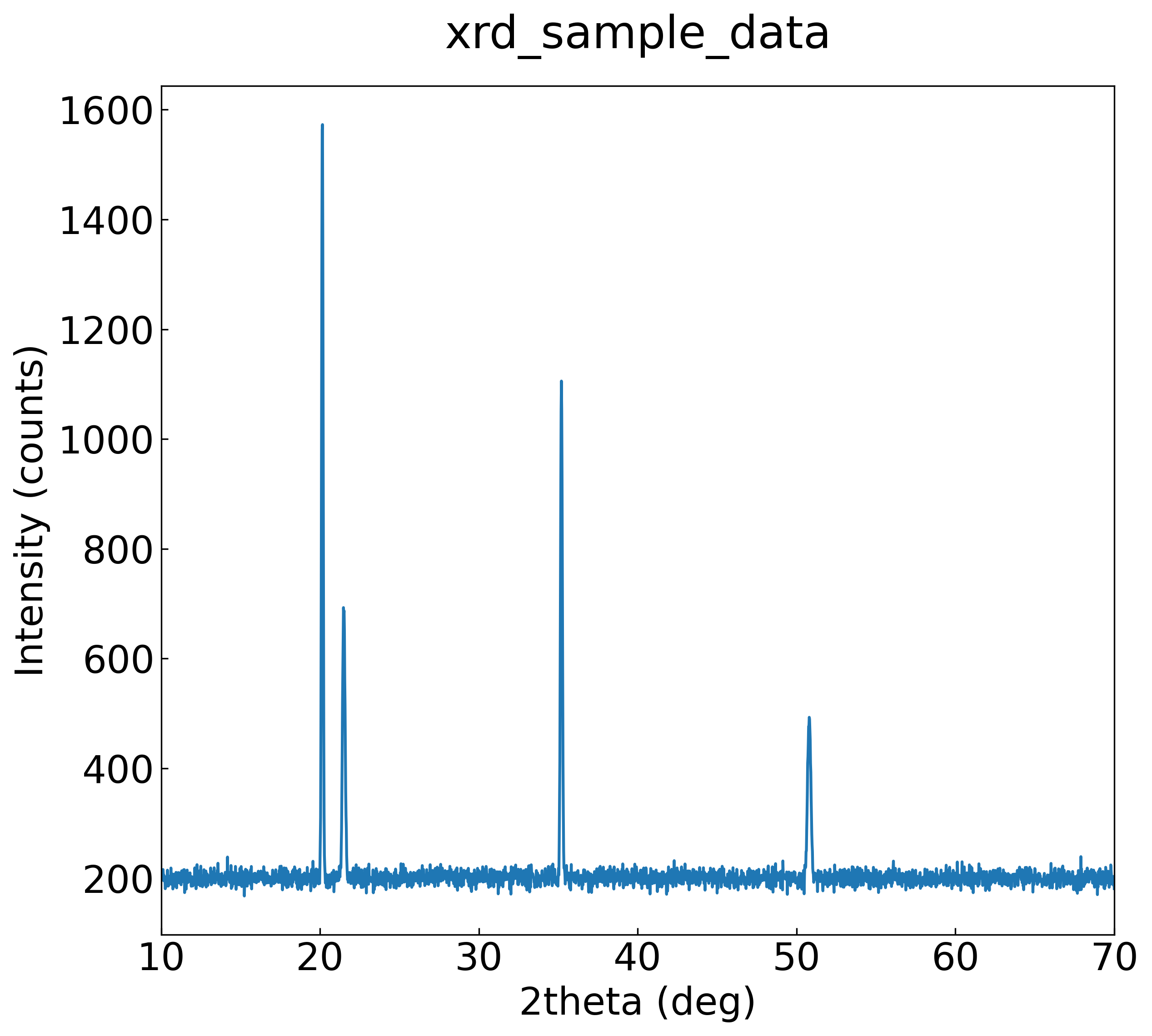
This minimal example plots XRD intensity data and uses --no-individual so that only the overlay image is produced (pass --individual to force per-series images even on single-series CSVs).
Data Overview
The dataset emulates XRD intensity measurements.
1 2 3 4 5 6 7 8 9 10 | |
Directory Layout
1 2 3 4 | |
How to Run
Switch between the Python script and CLI examples using the tabs below.
1 2 3 4 5 6 7 8 9 10 | |
1 | |
Option Details
no_individual=True,--no-individual: Skip individual plots and emit only the overlay image.
Sample 2: Log-Scale Y Axis
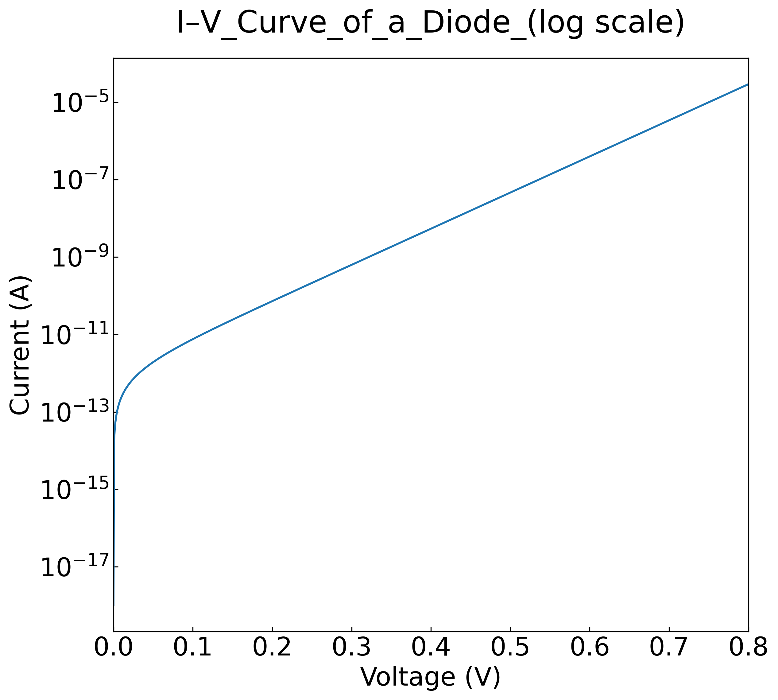
This sample uses synthetic diode I-V data to show how --logy plots the Y axis on a logarithmic scale while setting a custom title.
Data Overview
The dataset approximates the I-V characteristics of a diode.
1 2 3 4 5 6 7 8 9 10 | |
Directory Layout
1 2 3 | |
How to Run
Switch between the Python script and CLI examples using the tabs below.
1 2 3 4 5 6 7 8 9 10 11 | |
1 2 3 4 | |
Option Details
no_individual=True,--no-individual: Skip individual plots and emit only the overlay image.--logy/logy=True: Plot the Y axis on a logarithmic scale.
The sample dataset does not cover logarithmic X axes, but you can enable it with
--logx/logx=True.
Sample 3: Axis Inversion (X/Y)
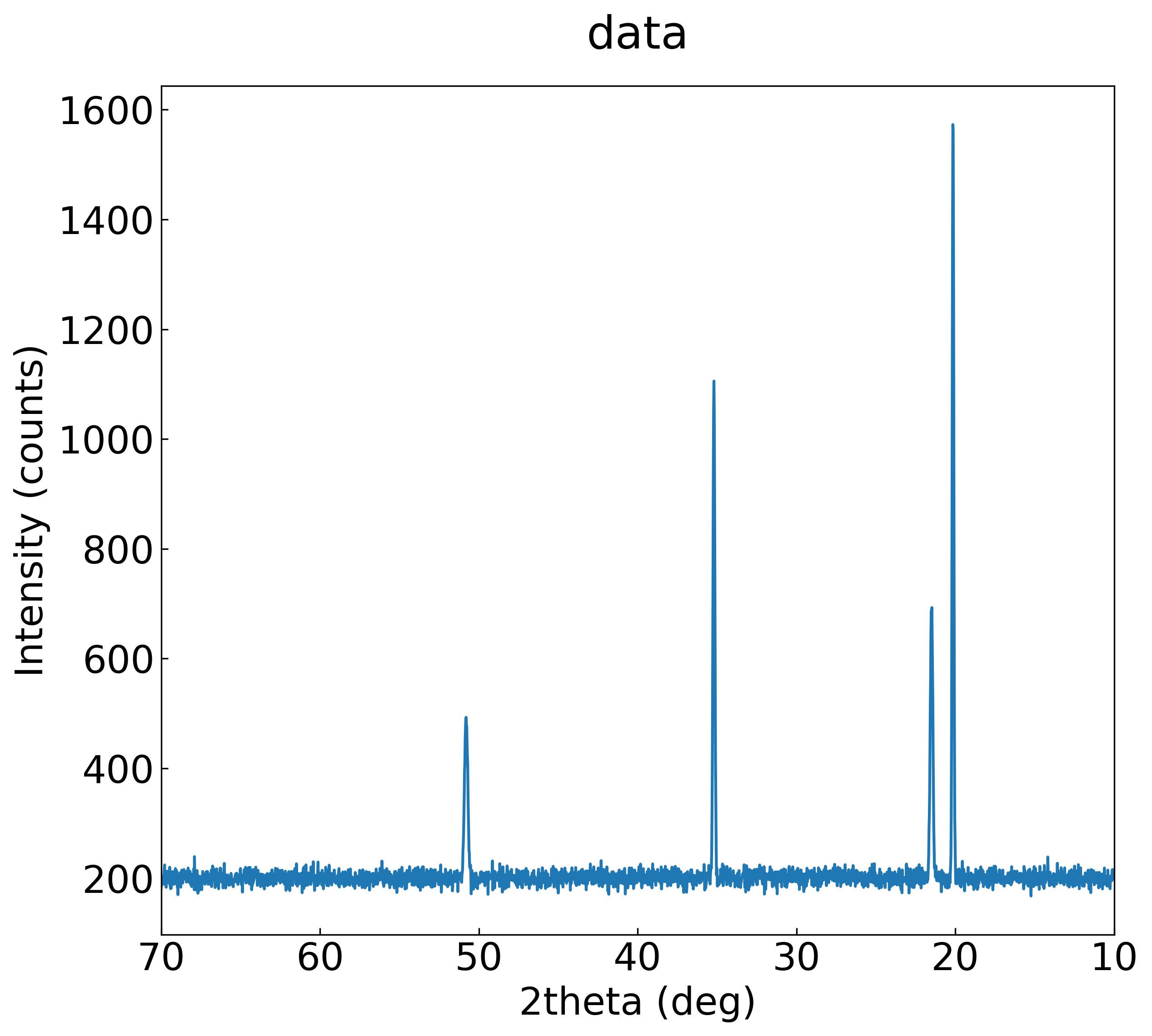
This example demonstrates --invert-x and --invert-y using XRD data.
Data Overview
The dataset emulates XRD intensity measurements.
1 2 3 4 5 6 7 8 9 10 | |
Directory Layout
Before running the sample, the directory contains:
1 2 3 | |
Inverting the X Axis
Switch between the Python script and CLI examples using the tabs below.
1 2 3 4 5 6 7 8 9 10 11 12 | |
1 | |
Inverting the Y Axis
1 2 3 4 5 6 7 8 9 10 11 | |
1 | |
Option Details
invert_x=True,--invert-x: Flip the overlay horizontally.invert_y=True,--invert-y: Flip the overlay vertically.no_individual=True: Skip individual plots and emit only the overlay image.
Sample 4: Overlaying Multiple X/Y Pairs
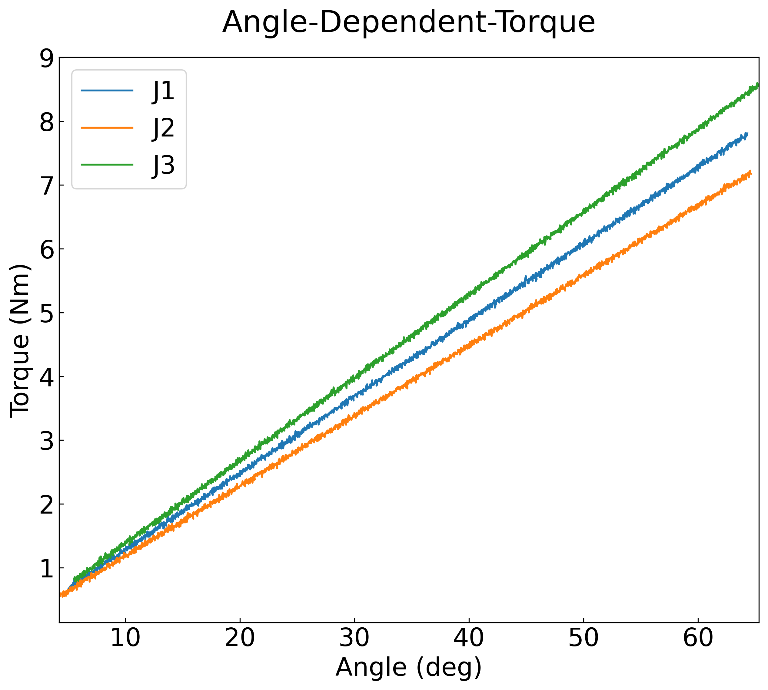
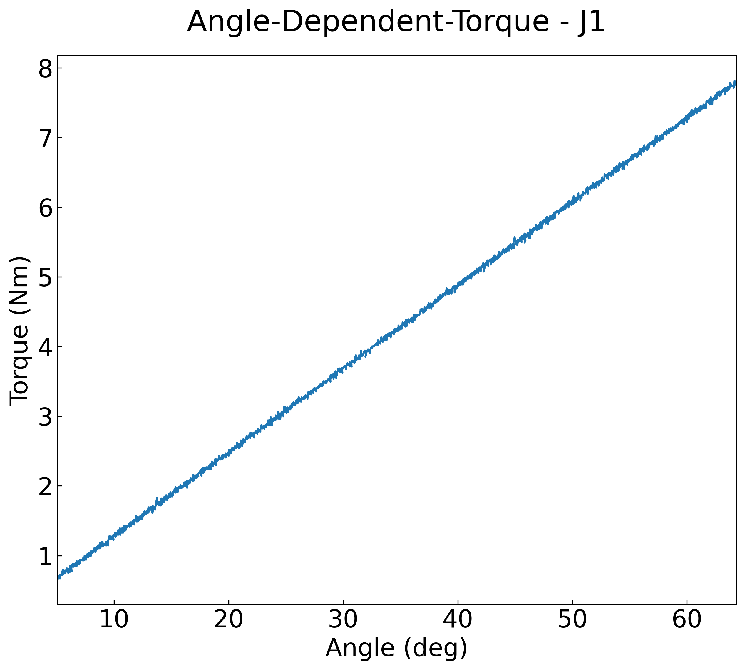
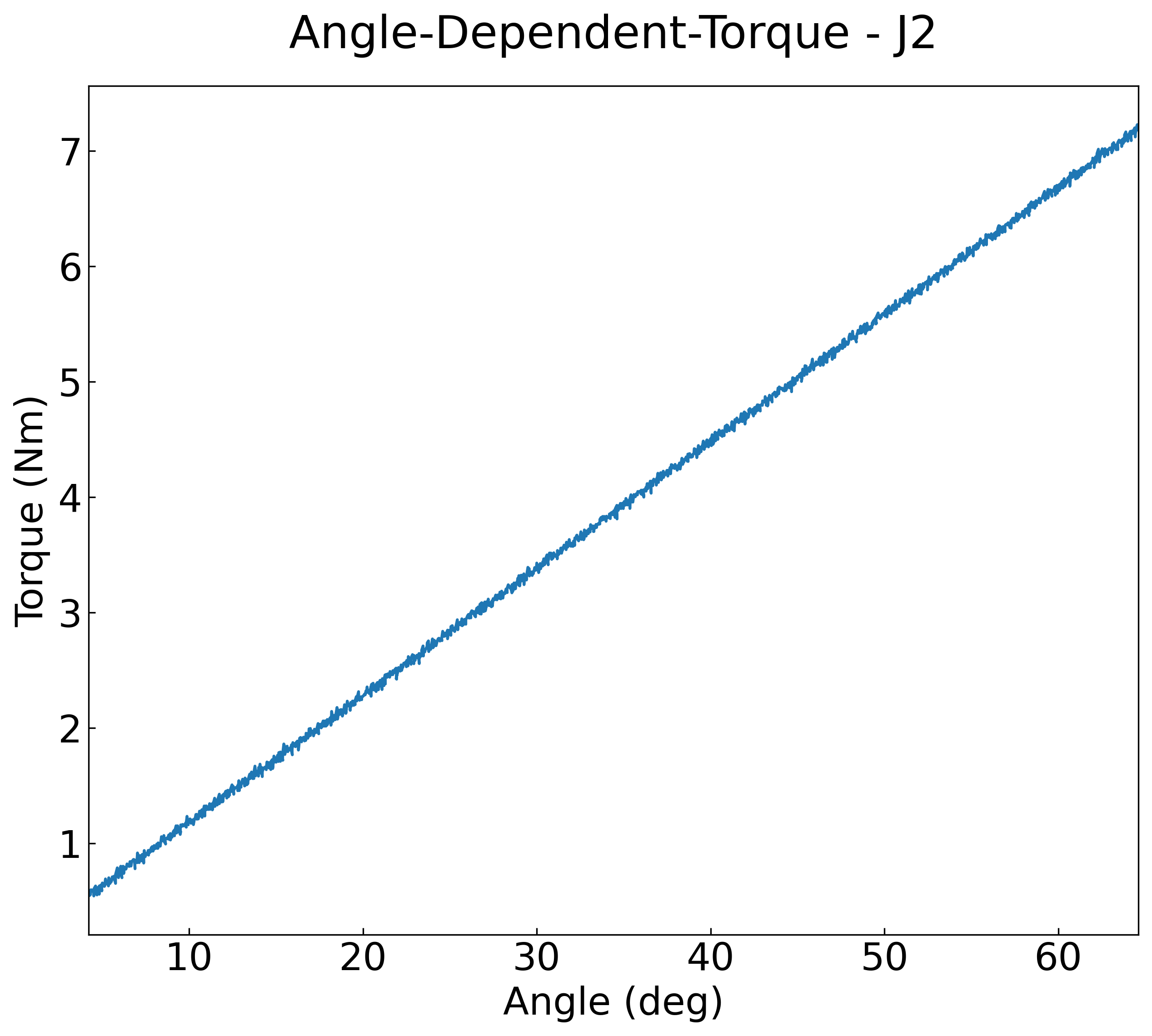
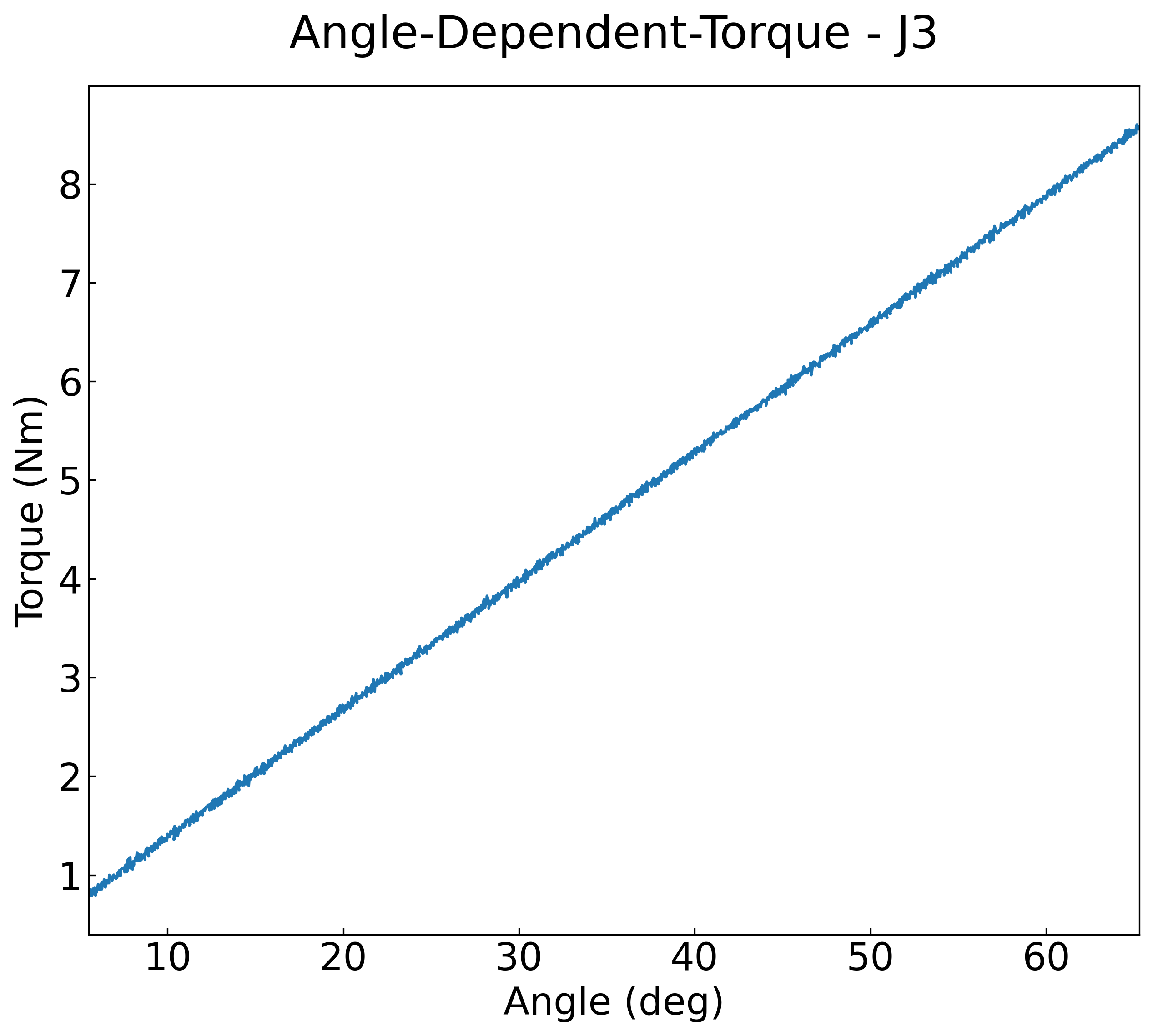
This sample plots three joint torque signals by pairing multiple X and Y columns and exports both the overlay and per-series plots.
Data Overview
Synthetic three-joint (J1-J3) angle/velocity/torque data generated from near-monotonic angles with a linear model plus small noise.
1 2 3 4 5 6 | |
Directory Layout
Before running the sample, the directory contains:
1 2 3 | |
How to Run
Switch between the Python script and CLI examples using the tabs below.
1 2 3 4 5 6 7 8 9 10 11 12 13 | |
1 2 3 4 5 | |
Option Details
--mode overlay: Overlay all series in a single figure (equivalent to the legacy x1y1x2y2 mode).--x-col 1 --x-col 4 --x-col 7: Specify three X columns (0-based indices 1, 4, 7). Each pairs with the corresponding Y column below.--y-cols 0 --y-cols 3 --y-cols 6: Specify the matching Y columns (indices 0, 3, 6) to form three series.--title "Angle-Dependent Torque": Set the plot title and filename stem.
Sample 5: One X Column with Many Y Series
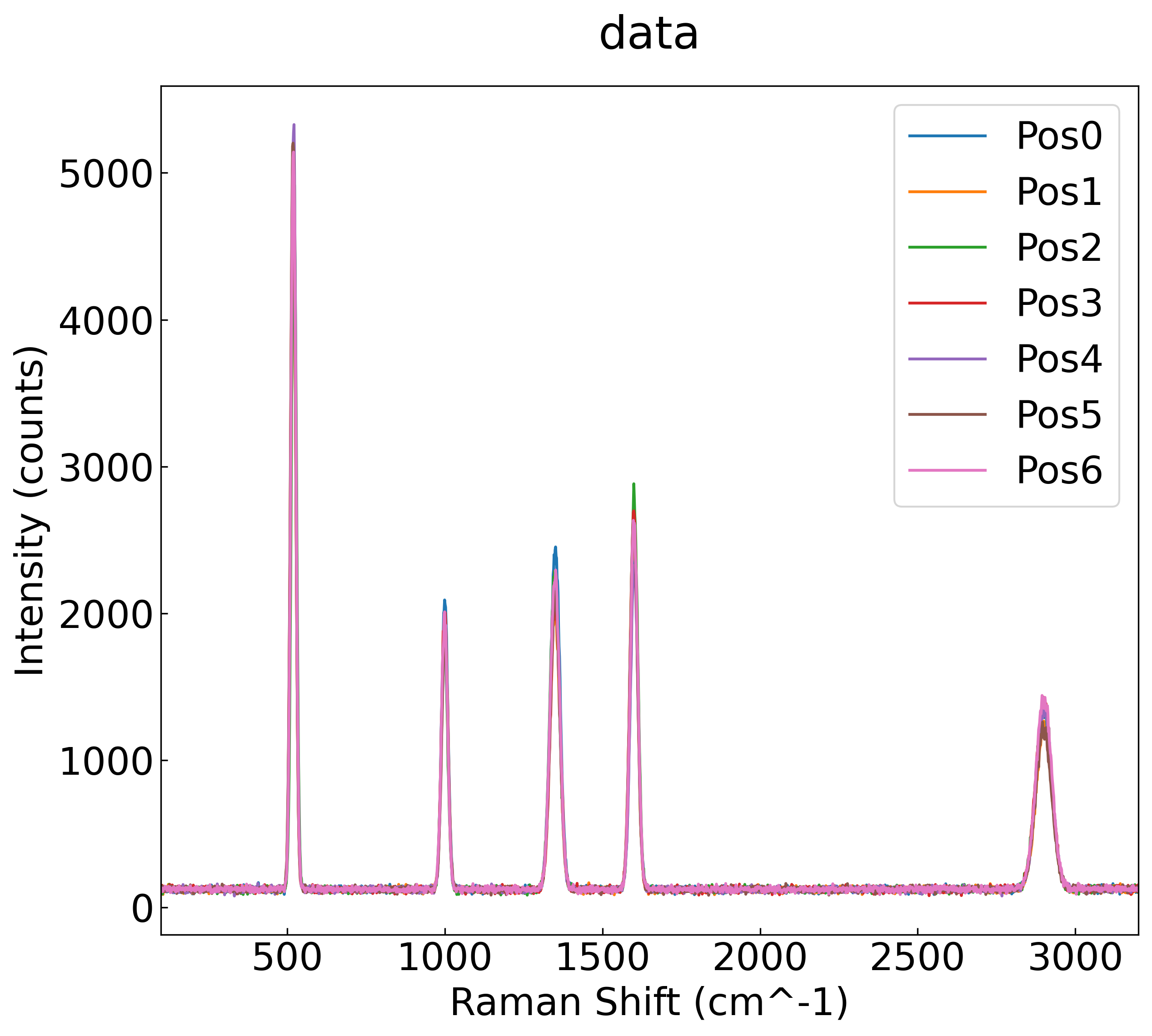
This Raman spectroscopy example pairs one X column with multiple Y series and customises the plot title.
Data Overview
Dummy Raman spectroscopy data. The horizontal axis is Raman Shift (cm^-1) and the Y series represent Intensity (counts) at positions Pos0-Pos10.
1 2 3 4 5 6 7 | |
Directory Layout
Before running the sample, the directory contains:
1 2 3 | |
How to Run
Switch between the Python script and CLI examples using the tabs below.
1 2 3 4 5 6 7 8 9 10 11 12 13 | |
1 2 3 4 5 | |
Option Details
--x-col 0: Use column 0 for the X axis. One declaration automatically pairs it with all specified Y columns.--y-cols 1 ... 5: Plot five Y series (columns 1-5).--no-individual: Output only the combined plot and skip individual PNGs.--title: Provide a custom plot title.
Sample 6: Limiting Legend Entries
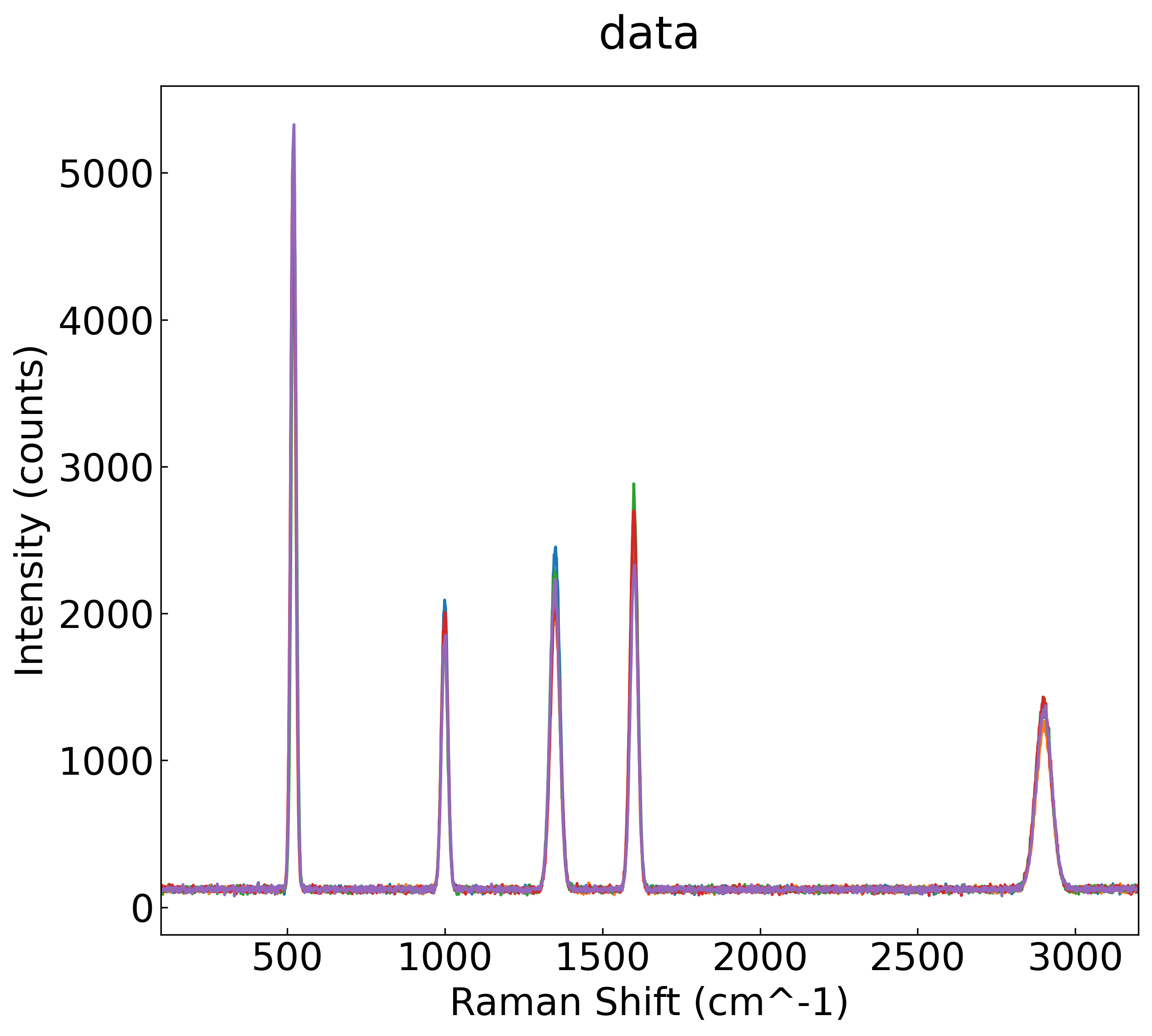
This Raman spectroscopy sample caps the number of legend items via --max-legend-items.
Data Overview
Dummy Raman spectroscopy data with Raman Shift (cm^-1) on the X axis and Intensity (counts) for positions Pos0-Pos10.
1 2 3 4 5 6 7 | |
Directory Layout
Before running the sample, the directory contains:
1 2 3 | |
How to Run
Switch between the Python script and CLI examples using the tabs below.
1 2 3 4 5 6 7 8 9 10 11 12 13 | |
1 2 3 4 5 | |
Option Details
--x-col 0: Use column 0 for the X axis so every declared Y column automatically pairs with it.--y-cols ...: Enumerate the five Y series (columns 1-5).--no-individual: Produce only the combined overlay PNG and skip per-series PNGs.--max-legend-items 3: Show at most three legend entries; remaining items are hidden to keep the plot readable.
Sample 7: Multi-Channel Charge/Discharge Overlay
This advanced example colours series by state labels spread across multiple columns while redirecting the output directory.
No pre-rendered images are bundled with this sample. Run the code to generate outputs.
Data Overview
The dataset mimics multi-channel charge/discharge measurements.
1 2 3 4 | |
How to Run
Switch between the Python script and CLI examples using the tabs below.
1 2 3 4 5 6 7 8 9 10 11 12 13 14 | |
1 2 3 4 5 6 7 8 | |
Option Details
--output-dir ./custom_output: Store generated PNG/HTML outputs in a custom folder instead of alongside the CSV.--title "Charge_Rest_Discharge": Set the plot title and filename stem (for example,Charge_Rest_Discharge.png).--mode overlay: Overlay all series in a single figure, pairing each X column with the corresponding Y column.--x-col 1--x-col 7 ... 43: Enumerate the X-axis columns (0-based). Here there are six series using columns 1, 7, 13, 19, 25, and 31.--y-cols 5 --y-cols 11 ... 47: List the matching Y columns (5, 11, 17, 23, 29, 35) in the same order as the X columns.--direction-cols 0,--direction-cols 6 ... 42: Provide the state/phase columns that control colouring or segmentation per series. Supply as many direction columns as Y series.--max-legend-items 5: Limit the legend to five entries so that additional series are hidden automatically.
Sample 8: Supplementary Legend Information
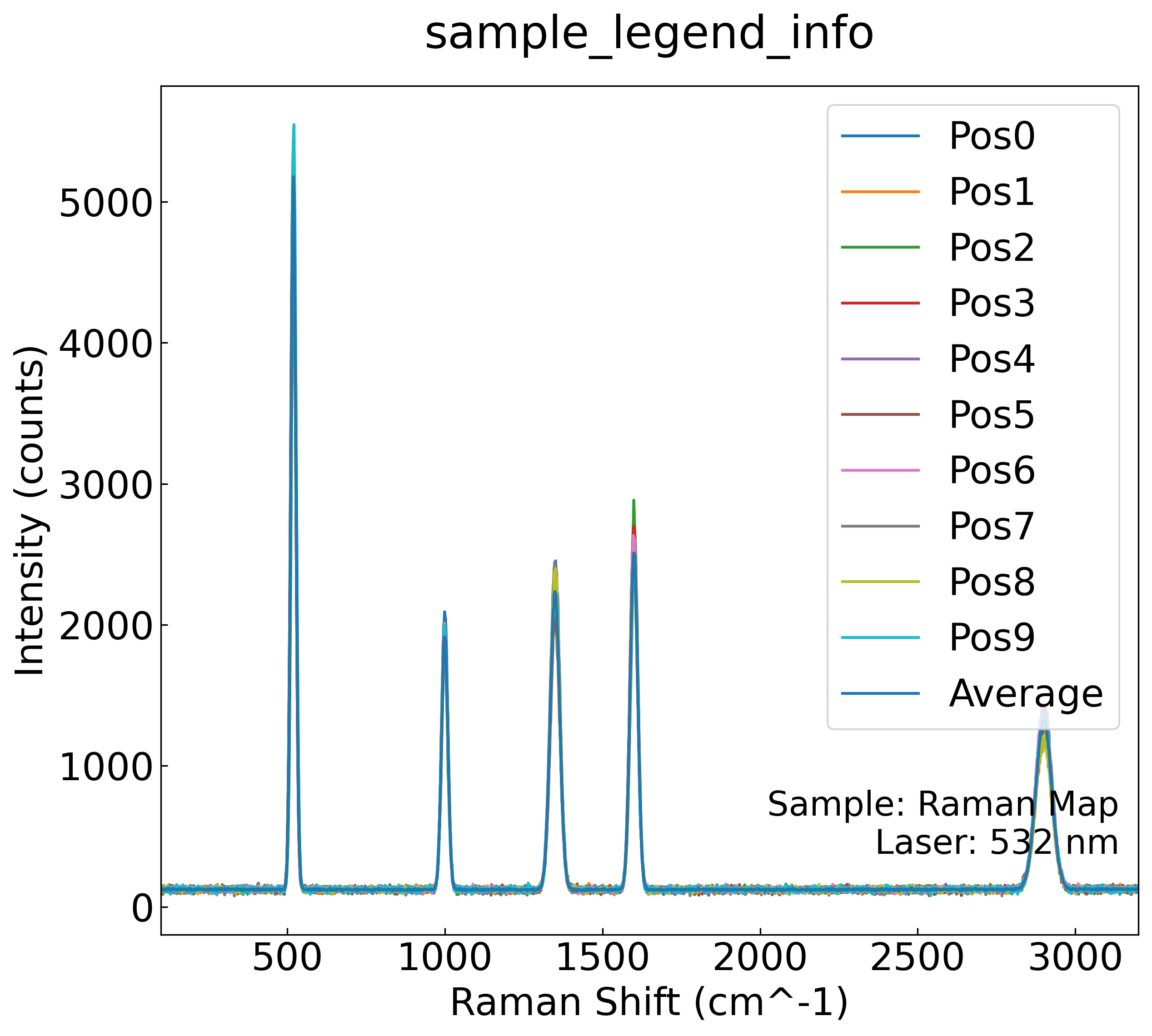
This sample appends extra metadata near the legend via --legend-info for Raman spectroscopy data.
Data Overview
Dummy Raman spectroscopy data with Raman Shift (cm^-1) on the X axis and Intensity (counts) for Pos0-Pos10.
1 2 3 4 5 6 7 | |
Directory Layout
Before running the sample, the directory contains:
1 2 3 | |
How to Run
1 2 3 4 5 6 7 8 9 10 11 | |
1 2 3 4 | |
Option Details
legend_info: Append arbitrary text near the legend (or in the upper right). Use\nto insert line breaks.no_individual=True: Generate only the overlay image and skip individual plots.
Sample 9: Displaying Grid Lines
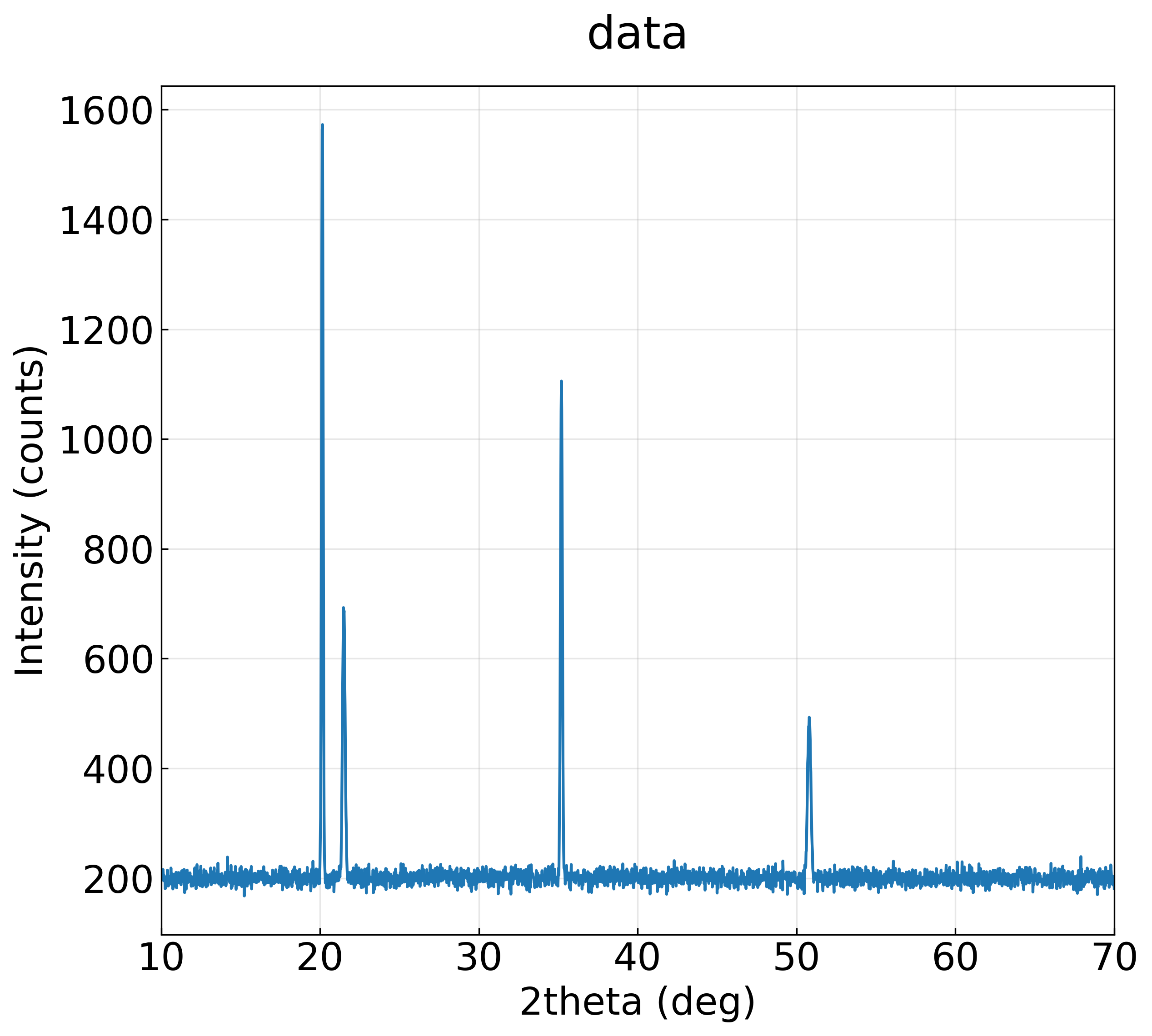
This XRD example enables grid lines with --grid to make peak locations easier to read.
Data Overview
The dataset uses synthetic XRD intensity values.
1 2 3 4 | |
Directory Layout
Before running the sample, the directory contains:
1 2 3 4 | |
How to Run
1 2 3 4 5 6 7 8 9 10 | |
1 2 3 | |
Option Details
grid=True,--grid: Draw horizontal and vertical grid lines to improve readability.no_individual=True: Skip individual plots and generate only the overlay image.
Sample 10: Narrowing the Display Range (xlim/ylim)
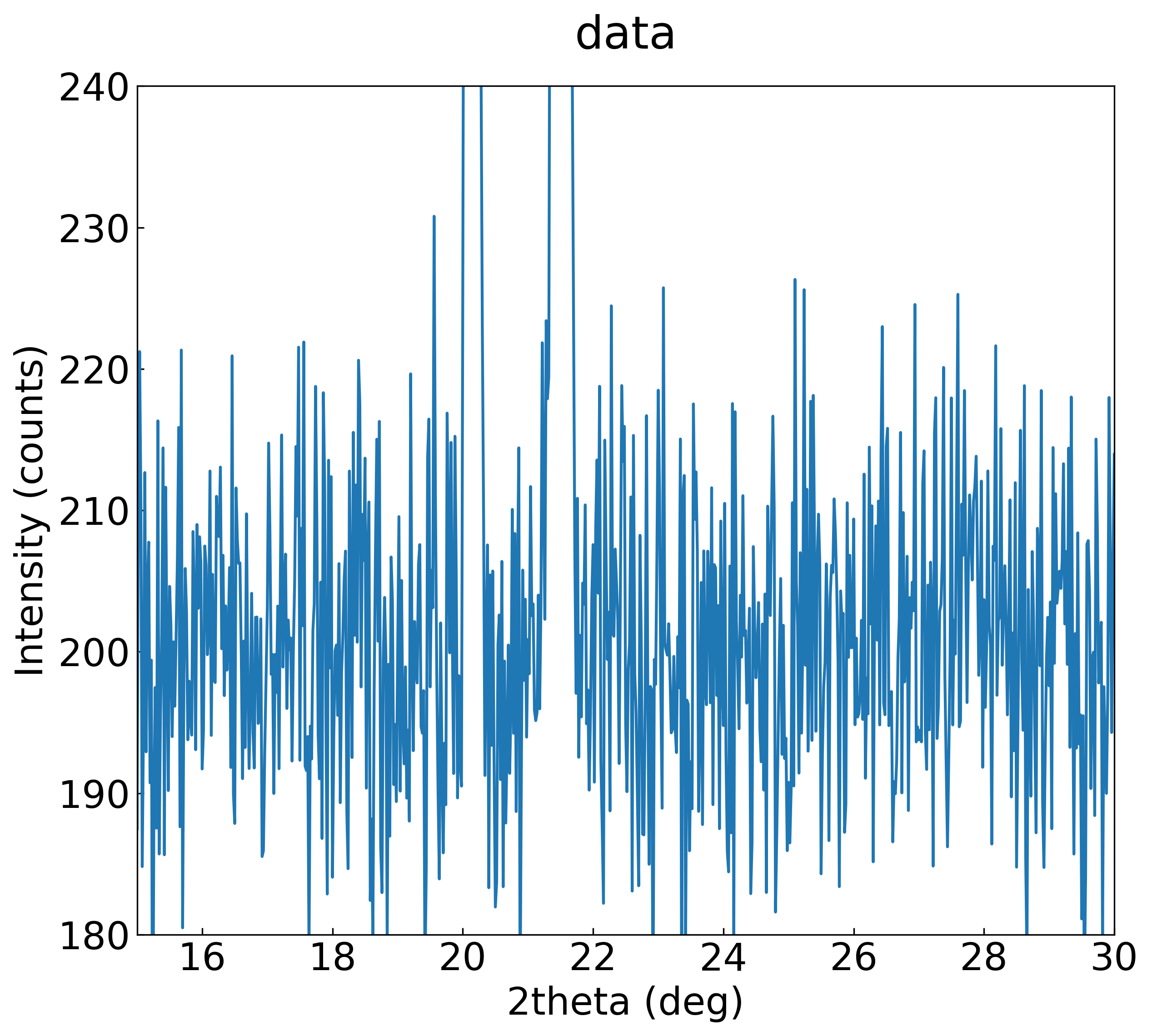
This sample zooms in on peak regions by combining --xlim and --ylim with XRD data.
Data Overview
The dataset reuses XRD intensity values and shows how to restrict the visible range.
1 2 3 4 | |
Directory Layout
Before running the sample, the directory contains:
1 2 3 4 | |
How to Run
1 2 3 4 5 6 7 8 9 10 11 | |
1 2 3 4 | |
Option Details
--xlim <min> <max>,xlim=(<min>, <max>): Restrict the X-axis range (same units as the CSV). The example displays only 2theta from 15 degrees to 30 degrees.--ylim <min> <max>,ylim=(<min>, <max>): Restrict the Y-axis range (same units as the dataset). The example keeps intensities between 180 and 240 counts.--no-individual: Produce only the overlay image and skip individual plots.
Zooming the range helps inspect peaks in detail and hide noisy regions.
Sample 11: Separating Overlay and Individual Outputs
This example saves the overlay image and individual series outputs in different directories via --main-image-dir and --output-dir.
Data Overview
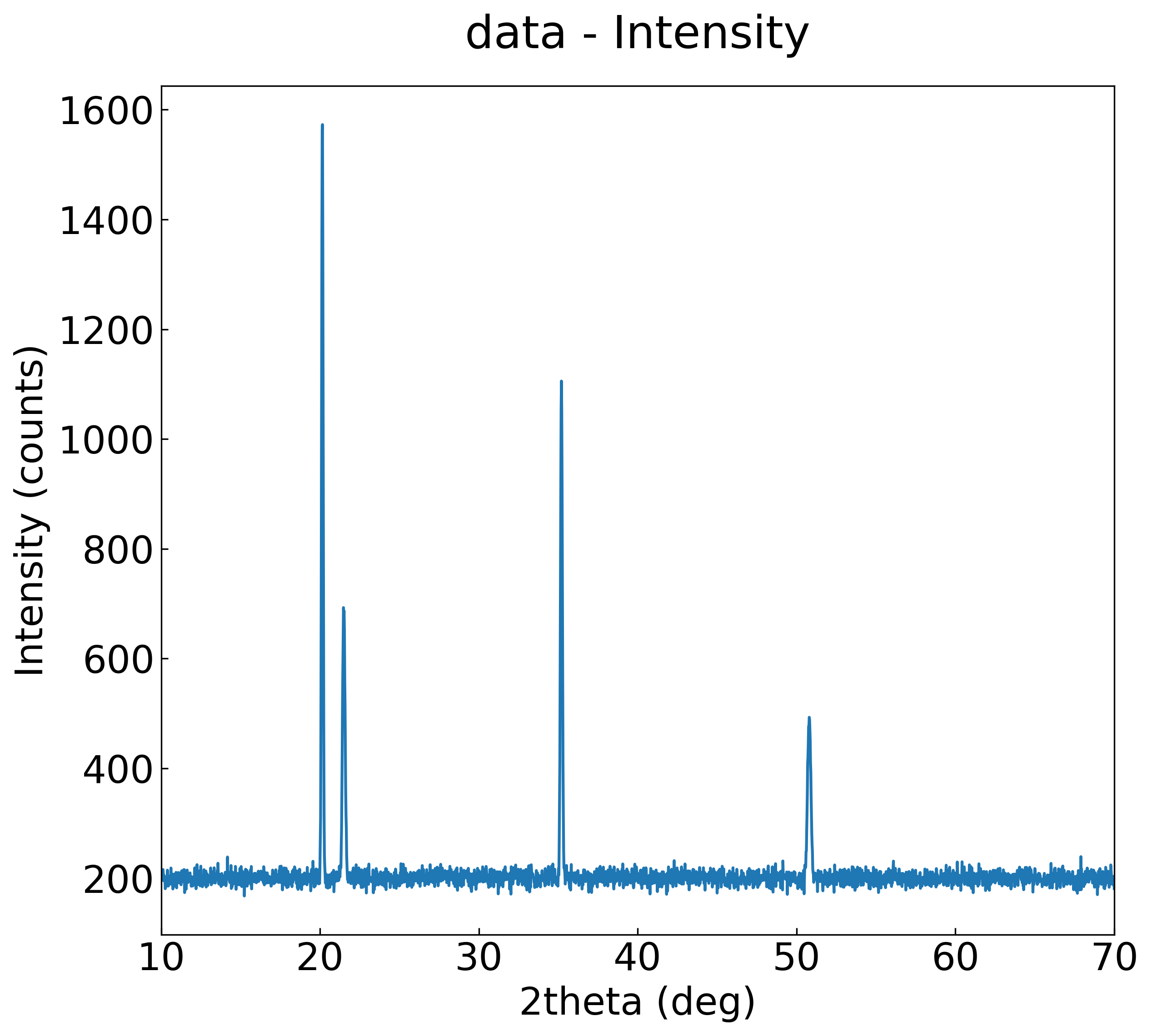
The dataset reuses synthetic XRD intensity data and demonstrates splitting output destinations.
1 2 3 4 | |
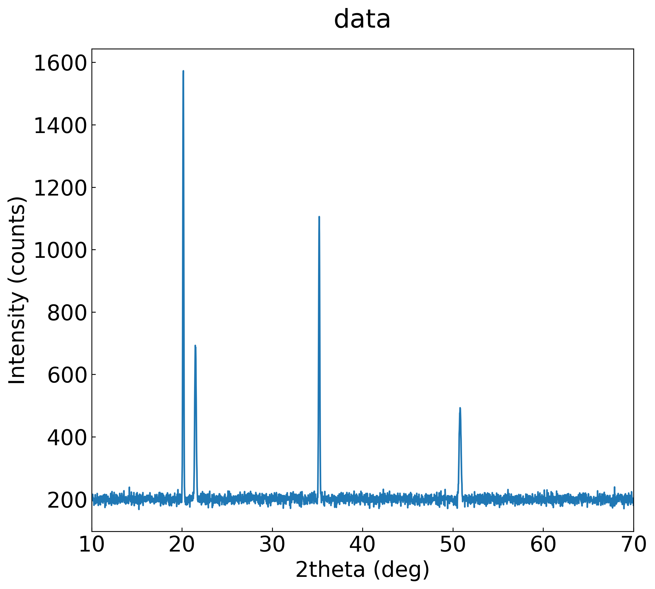
Directory Layout
1 2 3 4 | |
How to Run
1 2 3 4 5 6 7 8 9 10 | |
1 2 3 | |
Output Structure After Running
1 2 3 4 5 6 7 | |
Option Details
--main-image-dir: Choose where the overlay image is saved. By default it matches--output-dir.--output-dir: Choose where individual PNG and HTML outputs are saved. Without this option, outputs live next to the input CSV.
Separating the directories keeps report-ready overlays and detailed analysis plots organised.
Sample 12: Generating Plotly HTML Outputs
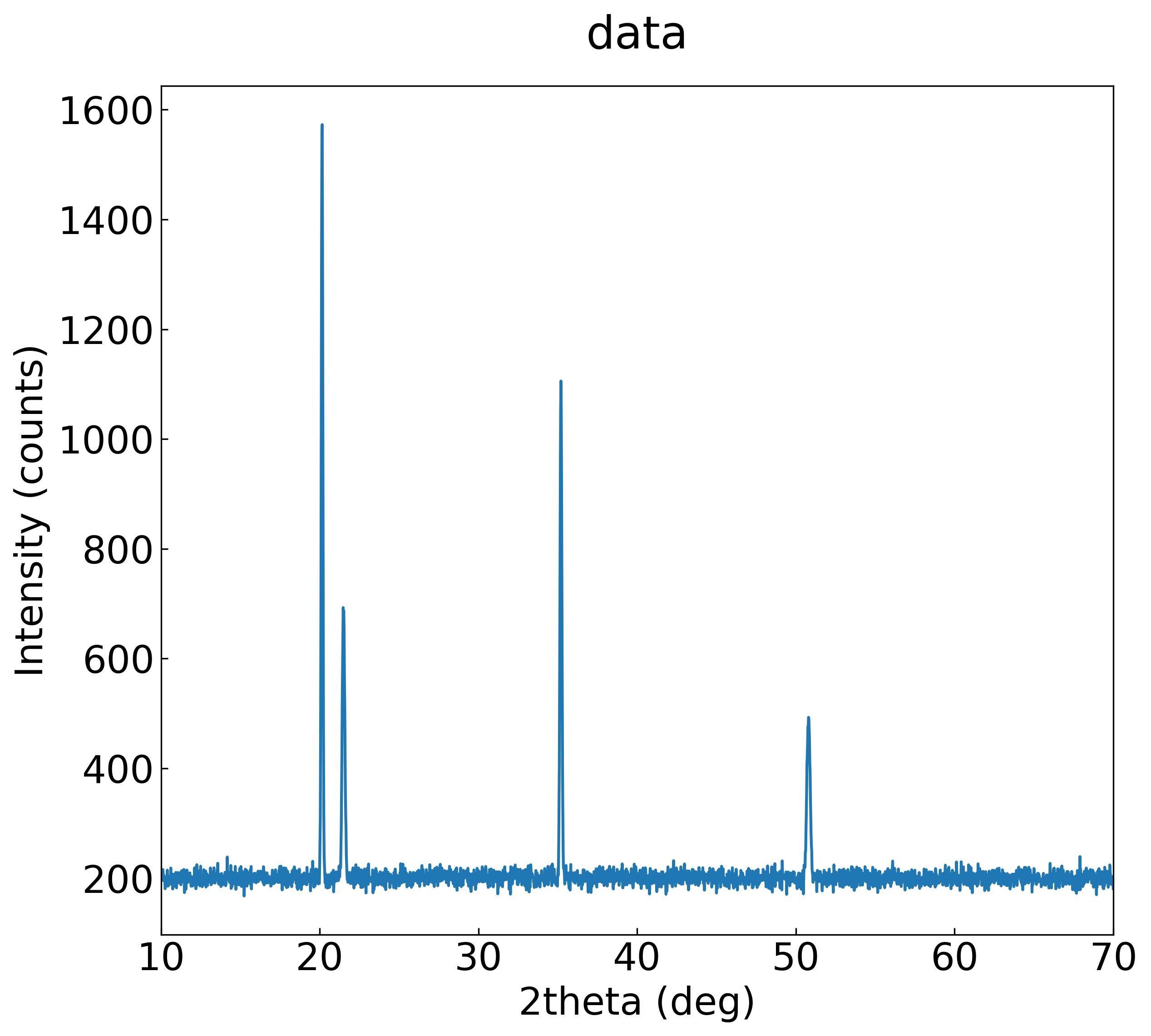
This sample enables interactive Plotly HTML output with --html.
Data Overview
Synthetic XRD intensity data used to demonstrate the Plotly export option.
1 2 3 4 | |
Directory Layout
1 2 3 | |
How to Run
1 2 3 4 5 6 7 8 9 10 | |
1 2 3 4 | |
Directory After Execution
1 2 3 4 5 6 | |
Option Details
--html: Produce interactive Plotly HTML files (*.html). Open them in a browser to zoom and inspect traces.--no-individual: Skip per-series plots and keep only the combined output (the HTML stays next to the CSV by default unless you pass--html-output-dir).
Plotly output requires the Plotly library. If it is missing, you will see the following error message:
1 2 3 | |
Sample 14: Choosing a Legend Placement Policy (legend_policy)
This sample compares how each legend_policy value (legacy / auto / inside / outside_right / outside_bottom / hide) places the legend, using dummy data with 12 and 3 series. See the "Legend placement policy" section in Visualizing CSV as Graphs for option details.
With outside_right / outside_bottom, the canvas is enlarged to fit the legend instead of shrinking the plot area, so the graph itself keeps its size even with many series.
Data Overview
The sample uses data.csv (12 series) and data_few.csv (3 series). Both contain monotonically increasing dummy series.
1 2 3 4 | |
- data.csv (12 series)
- data_few.csv (3 series)
Preparation: Generating the Dummy Data
The CSV files can be downloaded from the links above. To generate them locally, run the script below (the published data and figures were generated with it).
1 2 3 4 5 6 7 8 9 10 11 12 13 14 15 16 17 18 19 20 21 22 23 24 25 26 27 28 29 30 31 32 33 34 35 36 37 38 | |
1 | |
Directory Layout
1 2 3 4 5 | |
Running the bundled sample_legend_policy.py generates the PNGs for all cases below at once. The following sections show how to run each case individually.
Case 1: legacy (previous behavior)
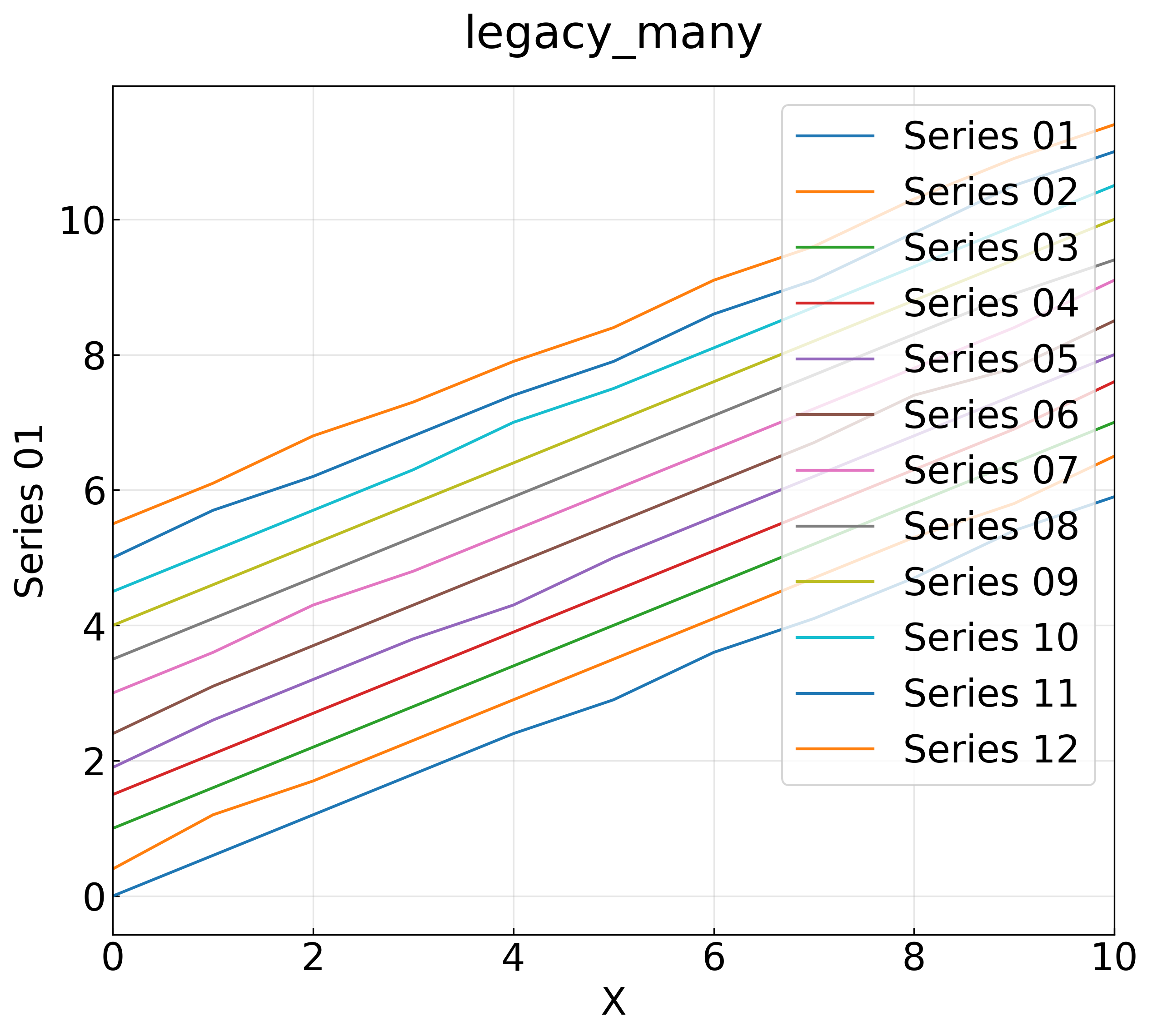
This is the default when legend_policy is not specified. The legend is rendered inside the plot area and controlled by legend_loc and max_legend_items as before.
1 2 3 4 5 6 7 8 9 10 11 12 13 14 15 | |
1 2 3 4 5 6 7 8 | |
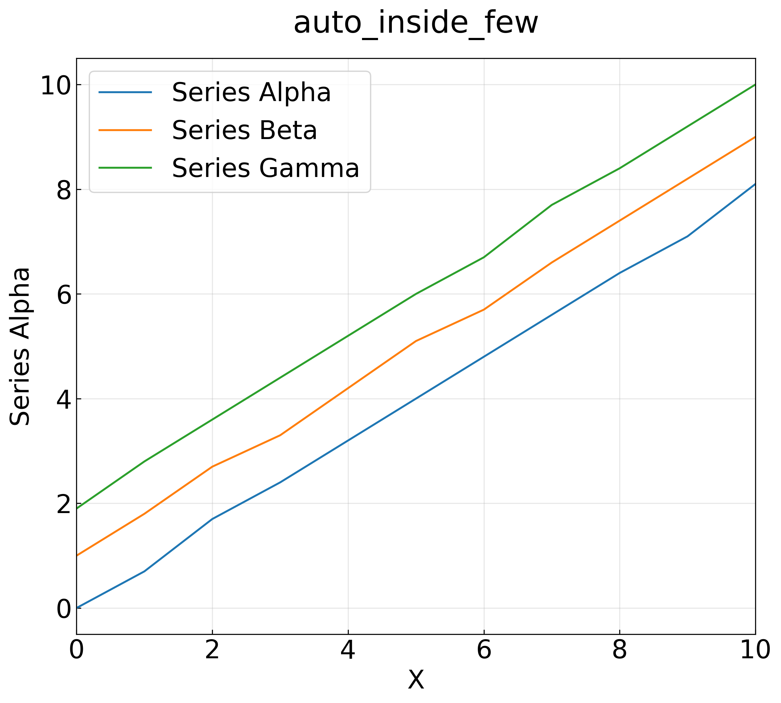
Case 2: auto with 3 series (kept inside)
auto picks the placement from the item count. Three series is at or below legend_outside_threshold (default 8), so the legend stays inside the plot area.
1 2 3 4 5 6 7 8 9 10 11 12 13 14 15 | |
1 2 3 4 5 6 7 8 | |
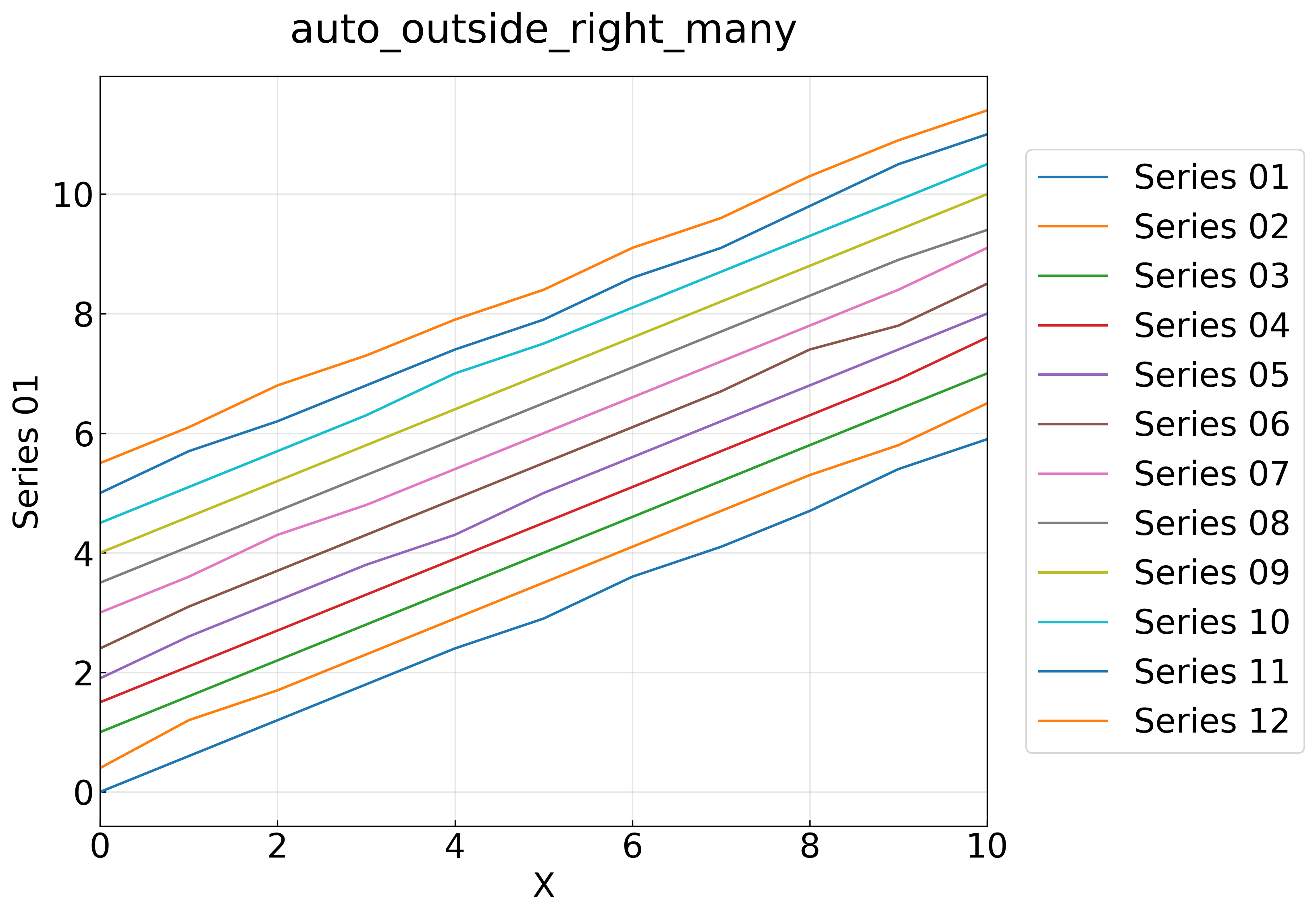
Case 3: auto with 12 series (switches to outside right)
Twelve series exceeds legend_outside_threshold=8, so auto moves the legend outside the plot on the right. The plot area keeps its size; the canvas grows to the right.
1 2 3 4 5 6 7 8 9 10 11 12 13 14 15 | |
1 2 3 4 5 6 7 8 | |
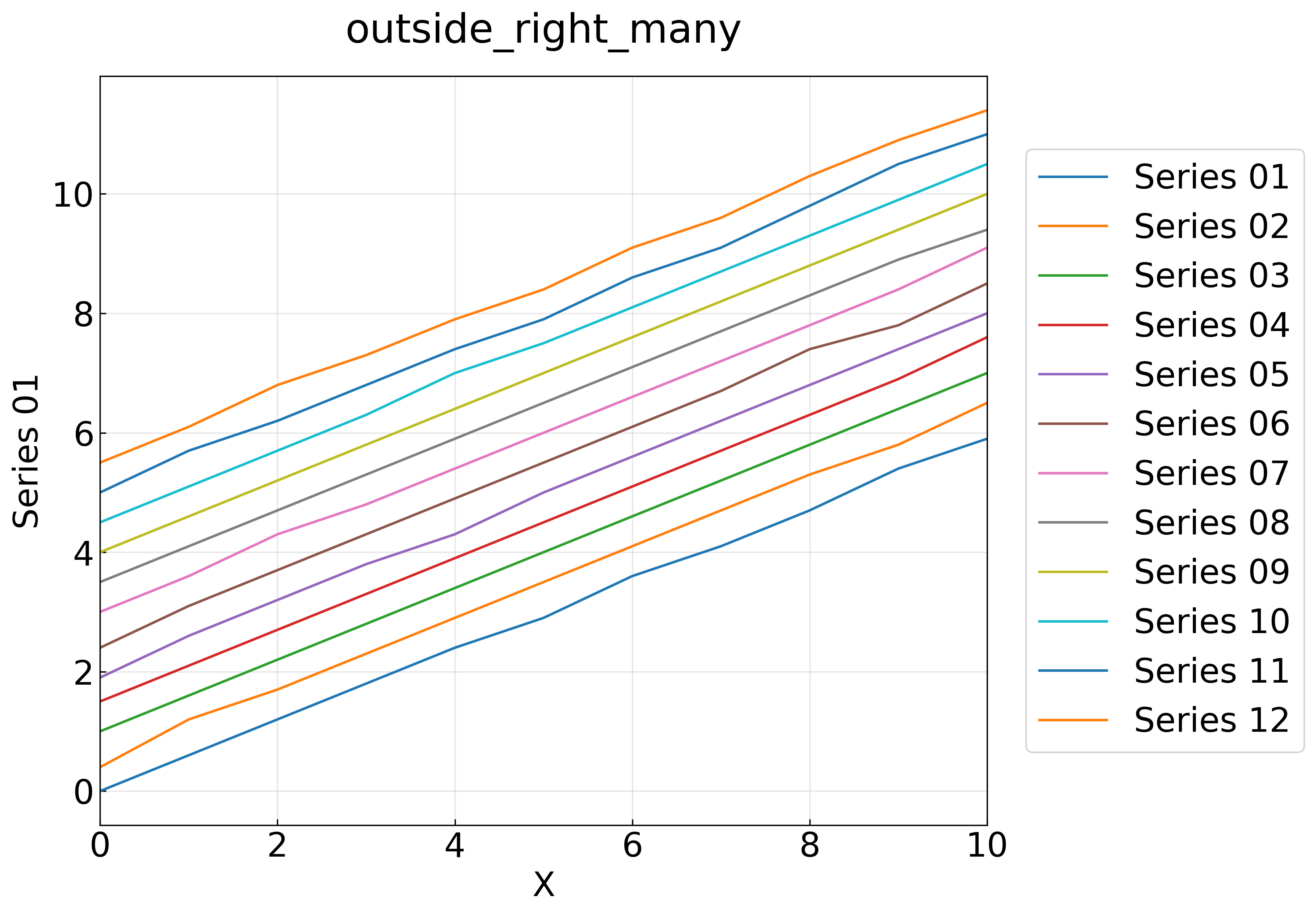
Case 4: Force outside_right
Places the legend outside the plot on the right regardless of the item count.
1 2 3 4 5 6 7 8 9 10 11 12 13 14 | |
1 2 3 4 5 6 7 | |
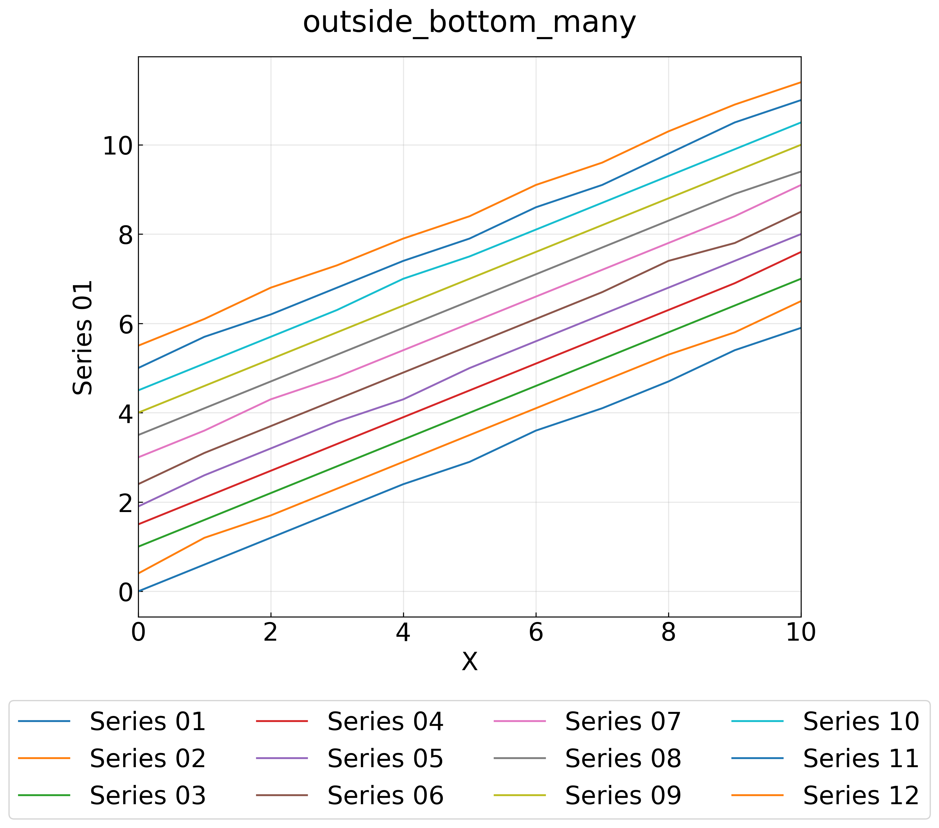
Case 5: outside_bottom with legend_ncol=4
Places the legend below the graph in 4 columns. The number of rows follows from the column count (12 items / 4 columns = 3 rows).
1 2 3 4 5 6 7 8 9 10 11 12 13 14 15 | |
1 2 3 4 5 6 7 8 | |
Case 6: hide (no legend)
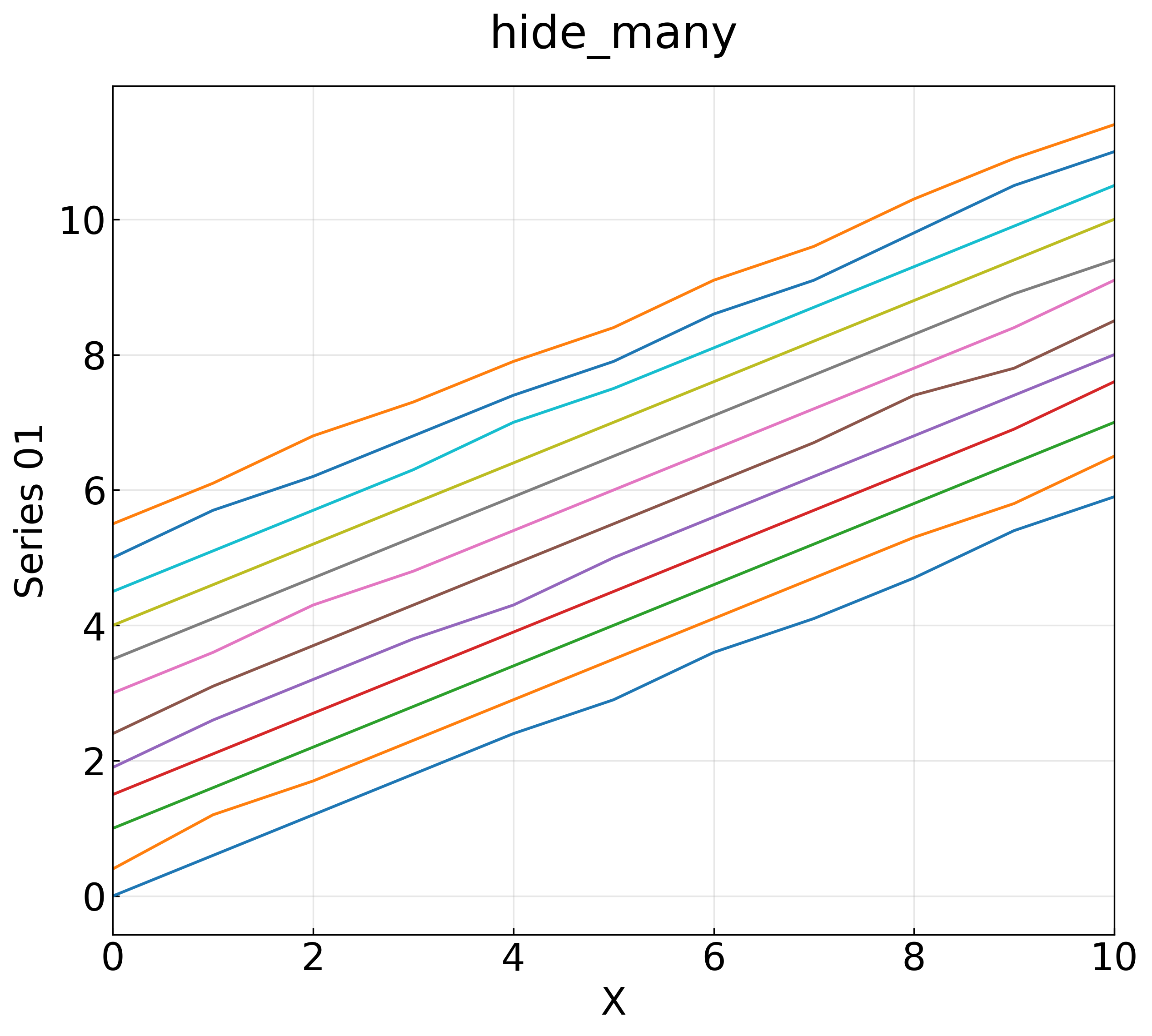
1 2 3 4 5 6 7 8 9 10 11 12 13 14 | |
1 2 3 4 5 6 7 | |
Case 7: auto exceeding max_legend_items (hidden automatically)
With max_legend_items=5 and 12 series, auto hides the legend because the cap is exceeded.
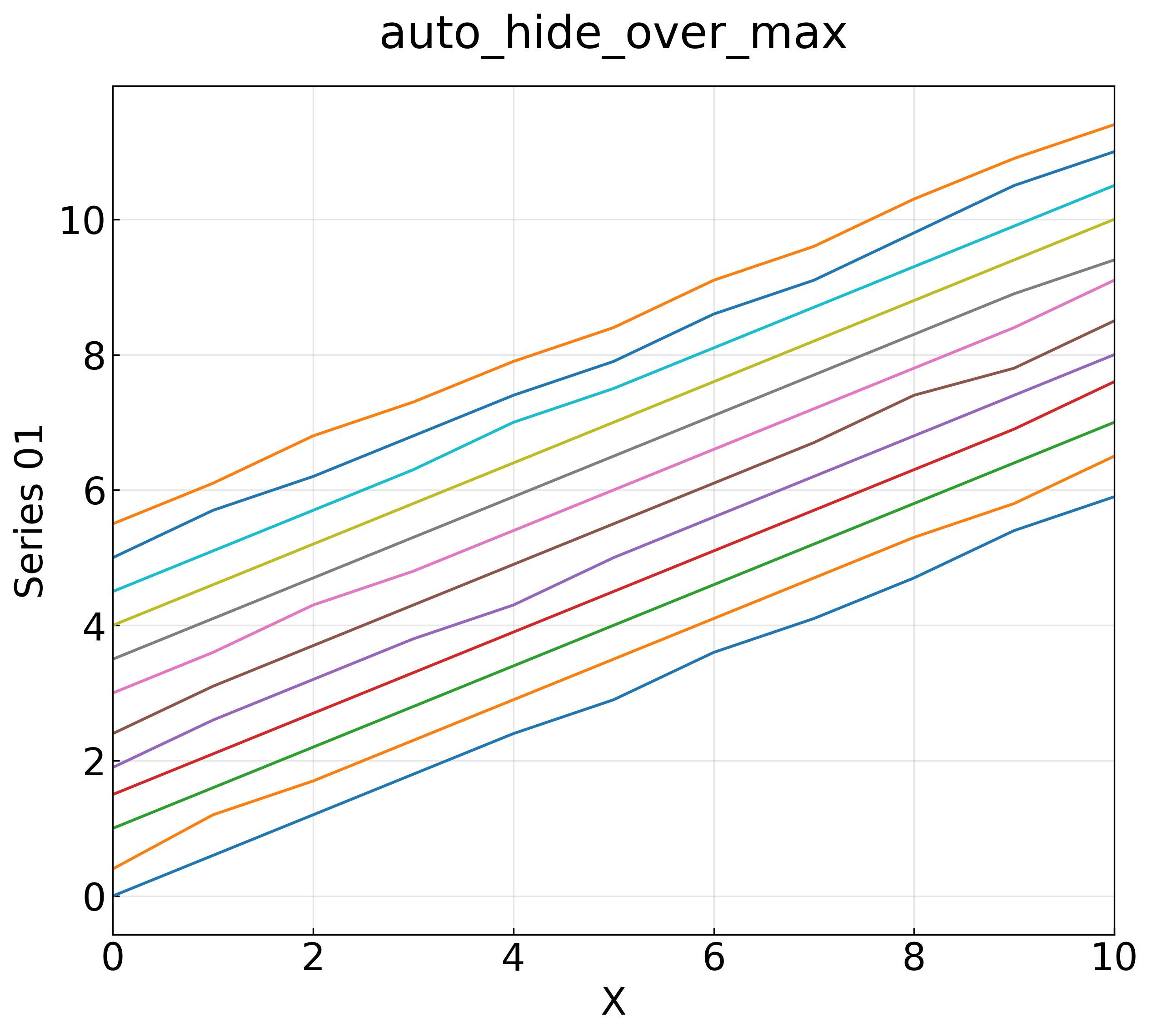
1 2 3 4 5 6 7 8 9 10 11 12 13 14 15 | |
1 2 3 4 5 6 7 8 | |
Option Details
legend_policy,--legend-policy: Legend placement policy. Choose fromlegacy(default, previous behavior) /auto(chosen from the item count) /inside/outside_right/outside_bottom/hide.legend_outside_threshold,--legend-outside-threshold: Item-count threshold at whichautoswitches from inside to outside-right placement (default 8; switches when exceeded).legend_ncol,--legend-ncol: Number of legend columns foroutside_bottom(3 when omitted).max_legend_items,--max-legend-items: Maximum number of legend items. The legend is hidden when exceeded (also applies to explicit non-autopolicies).x_col="x",--x-col x: Selects the X column by name. Wheny_colsis omitted, all remaining columns become Y series.
Sample 15: Dense Legends with 30+ Series and Automatic Placement
This sample uses dummy data with 32 series to demonstrate legend control when there are very many legend items. With legend_bottom_threshold (default 21), auto automatically places the legend below the graph at 21 or more items.
In every case the plot area keeps its size; the canvas is enlarged to fit the legend, and the legend is never clipped in the saved PNG/SVG files.
Data Overview
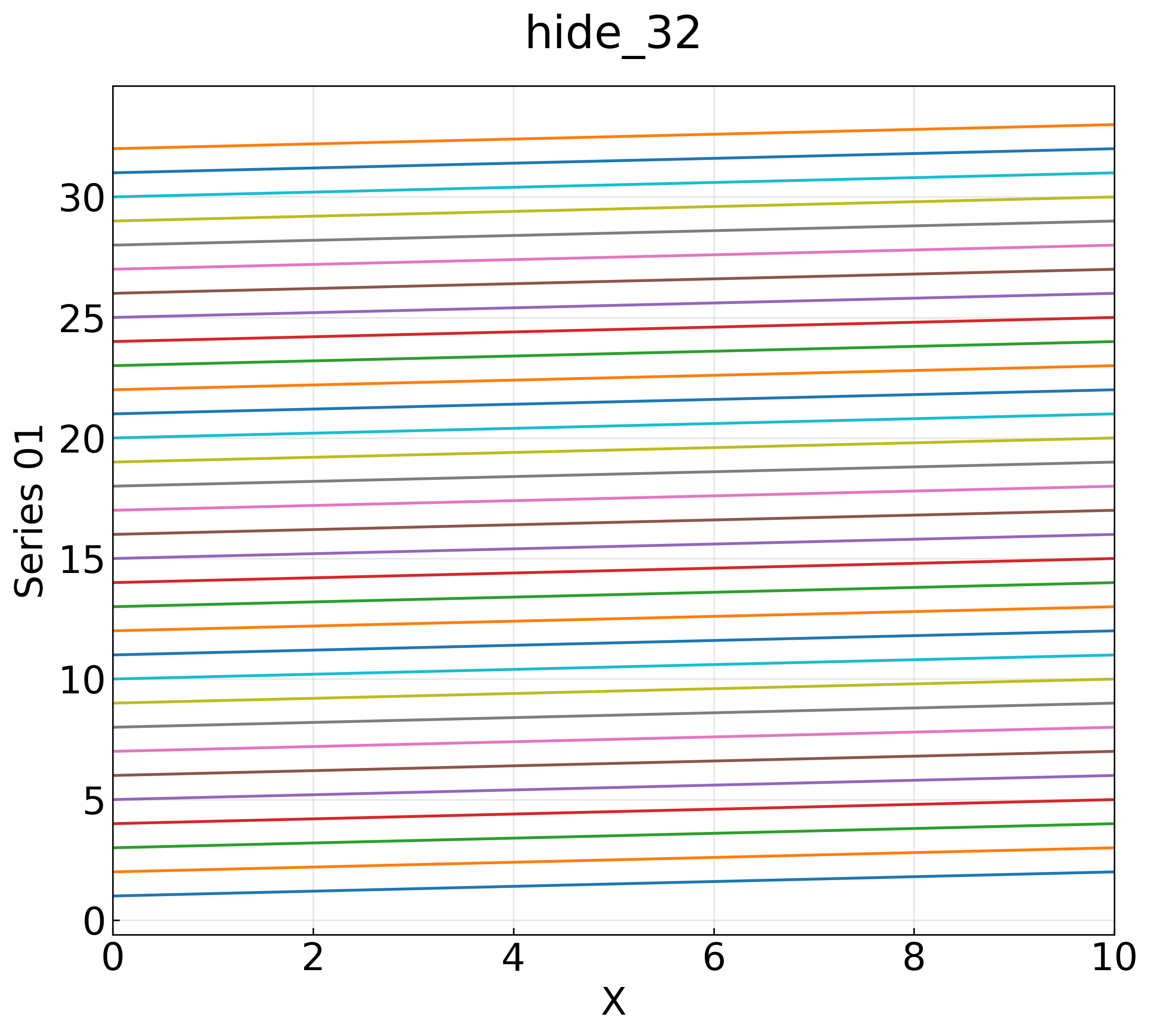
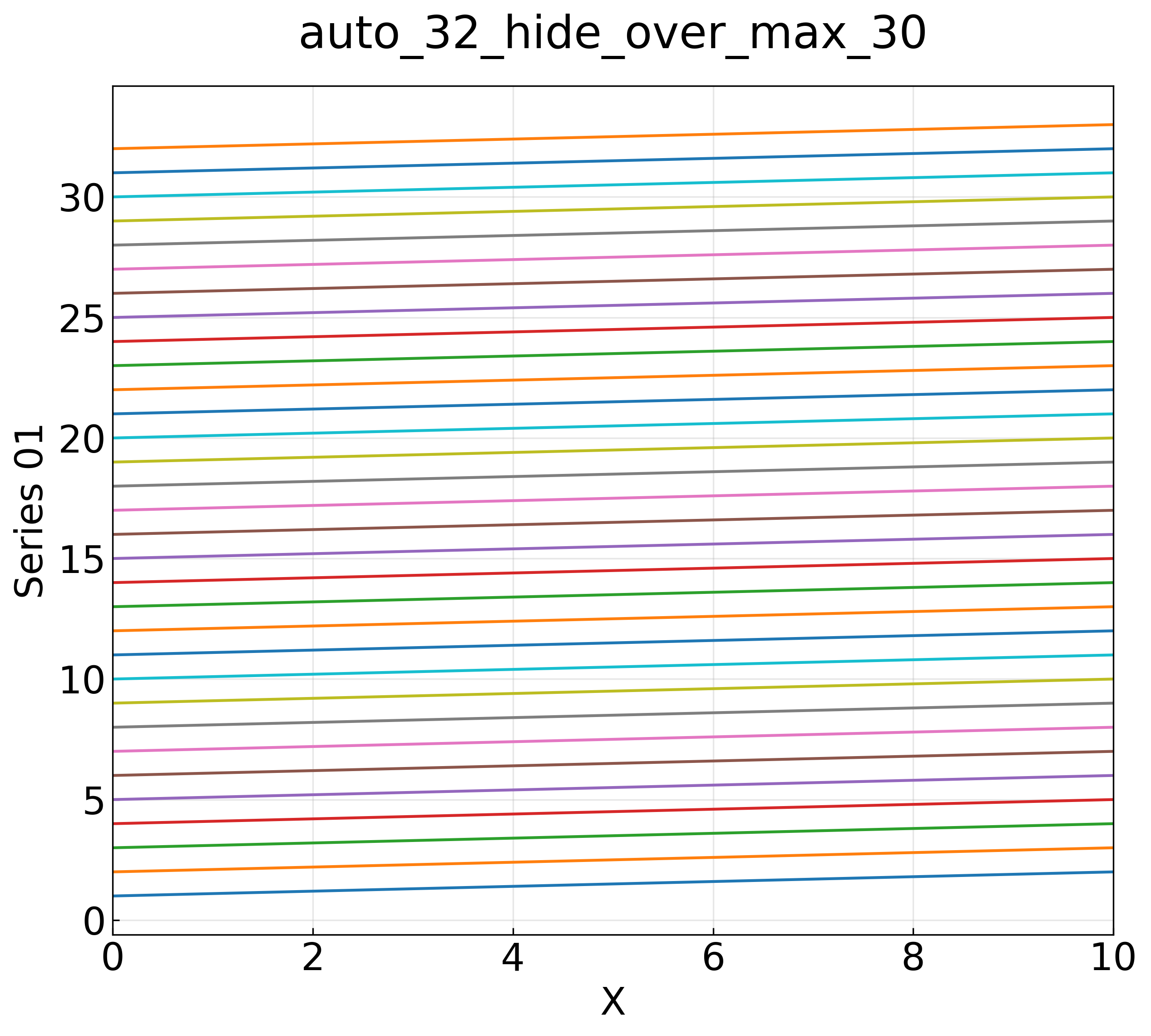
Straight-line data with 32 series. Each series is exactly series_i(x) = i + 0.1 * x (x = 0..10).
1 2 3 4 | |
- data.csv (32 series)
Preparation: Generating the Dummy Data
The script below reproduces the published CSV exactly.
1 2 3 4 5 6 7 8 9 10 11 12 13 14 15 | |
1 | |
Directory Layout
1 2 3 4 | |
Running the bundled sample_dense_legend.py generates the PNGs for all cases below at once.
Case 1: Default auto behavior (21+ items go below the graph)
Thirty-two series is at or above the default legend_bottom_threshold=21, so auto places the legend below the graph. The column count defaults to 3; pass legend_ncol=8 to compact it into 4 rows.
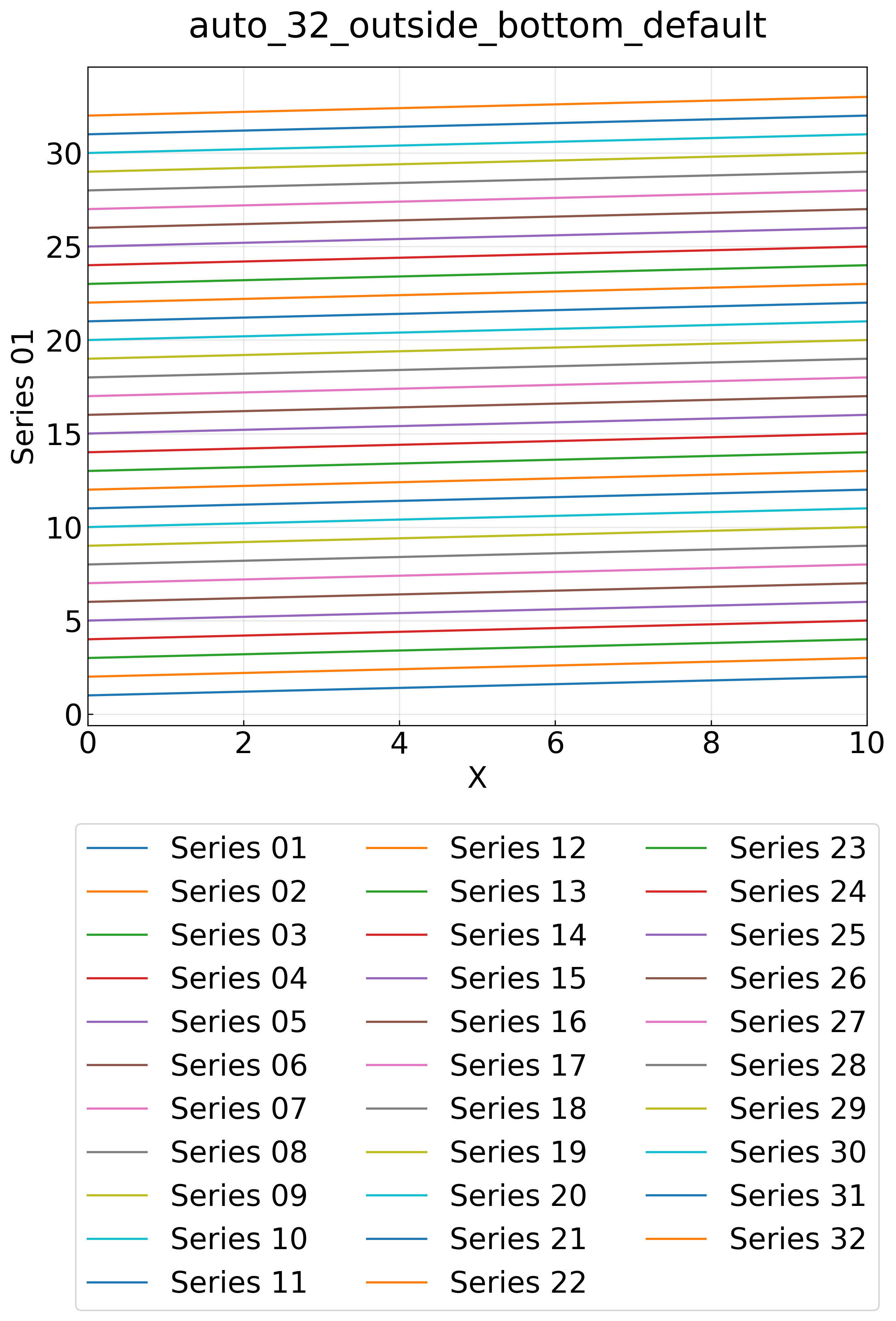
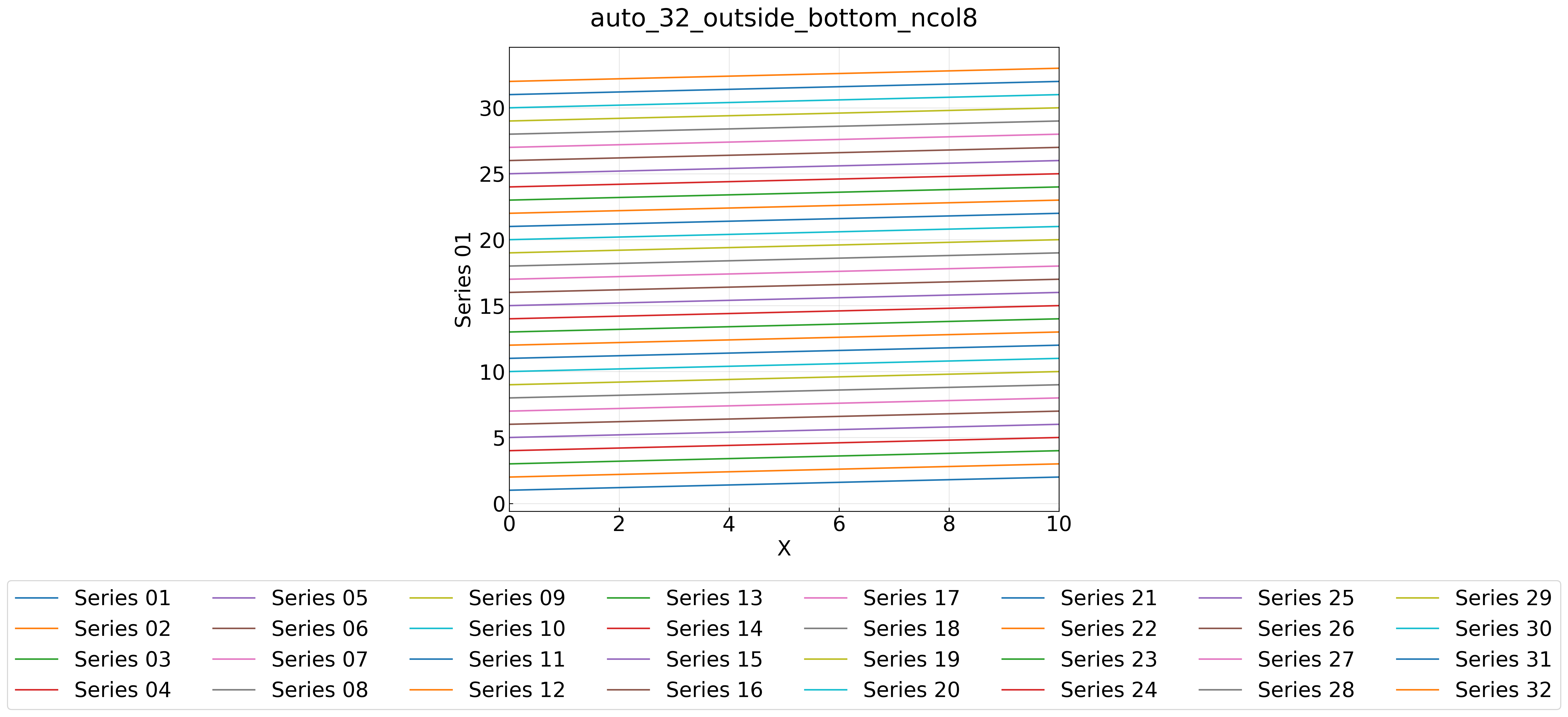
1 2 3 4 5 6 7 8 9 10 11 12 13 14 15 16 | |
1 2 3 4 5 6 7 8 9 | |
Case 2: Disable the bottom switch and keep the legend on the right
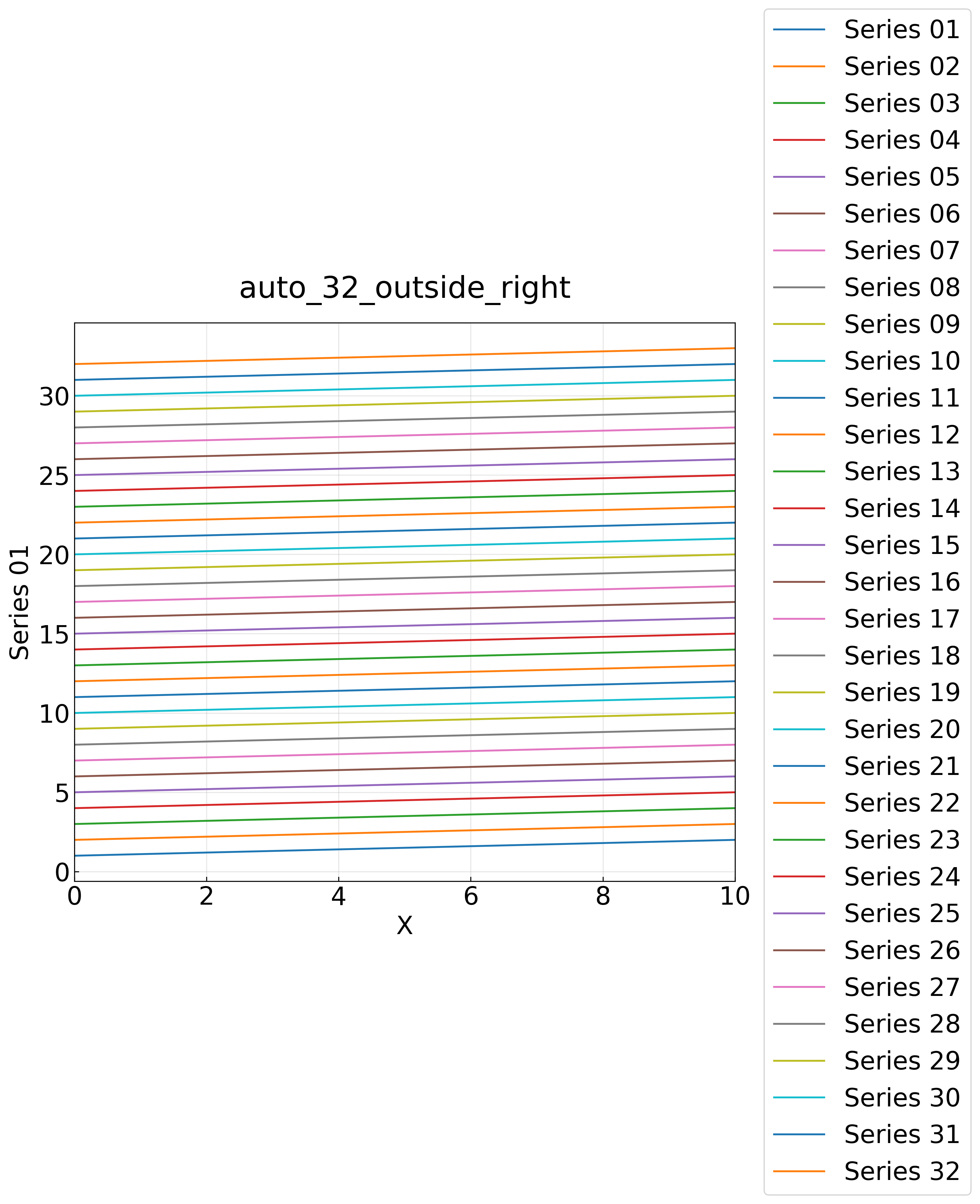
Passing legend_bottom_threshold=None (--legend-bottom-threshold 0 on the CLI) disables the automatic switch to bottom placement, so the legend goes outside on the right as before. Even a tall 32-item legend is not clipped because the canvas also grows vertically.
1 2 3 4 5 6 7 8 9 10 11 12 13 14 15 16 | |
1 2 3 4 5 6 7 8 9 | |
Case 3: Boundary behavior of legend_outside_threshold
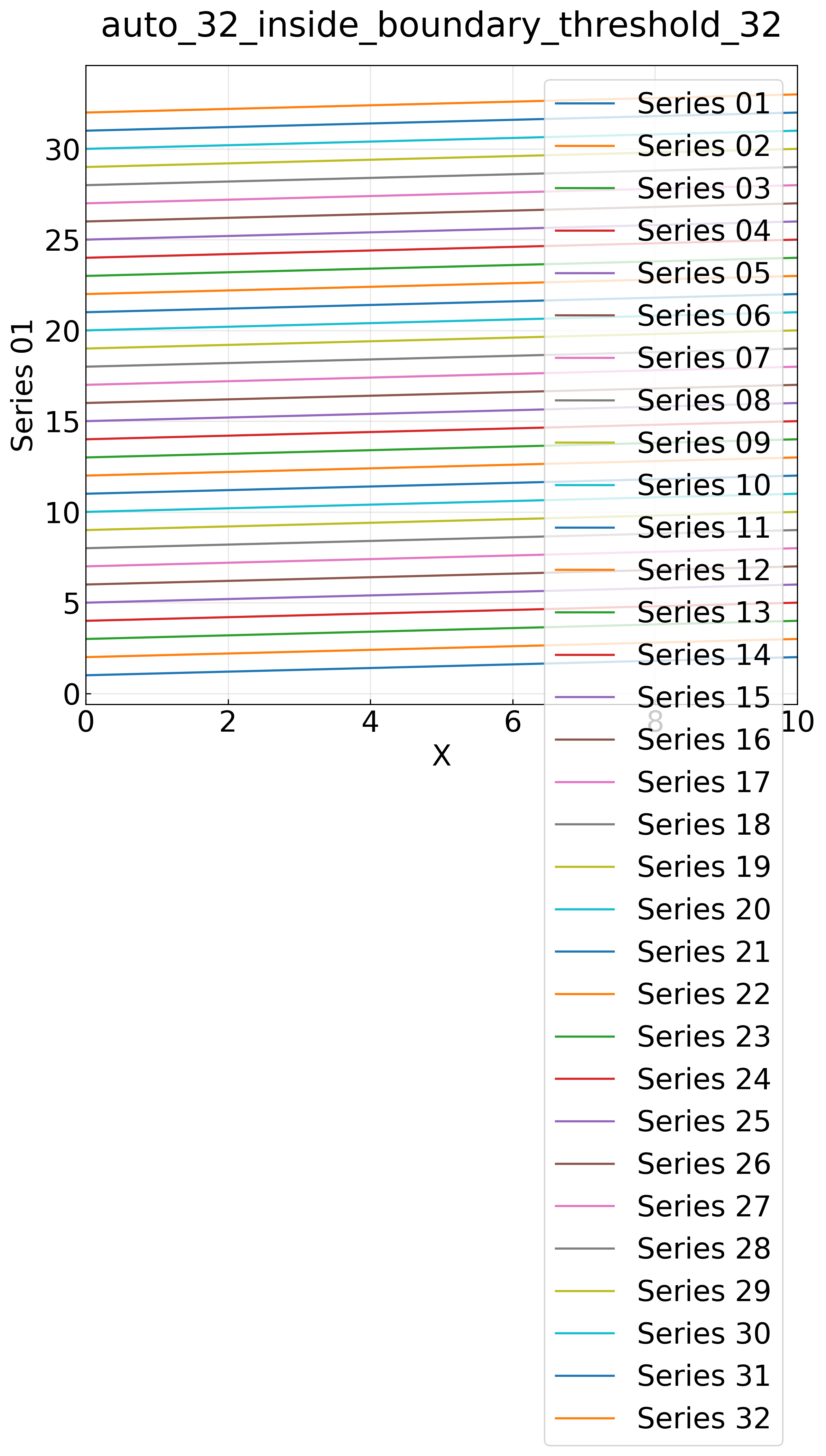
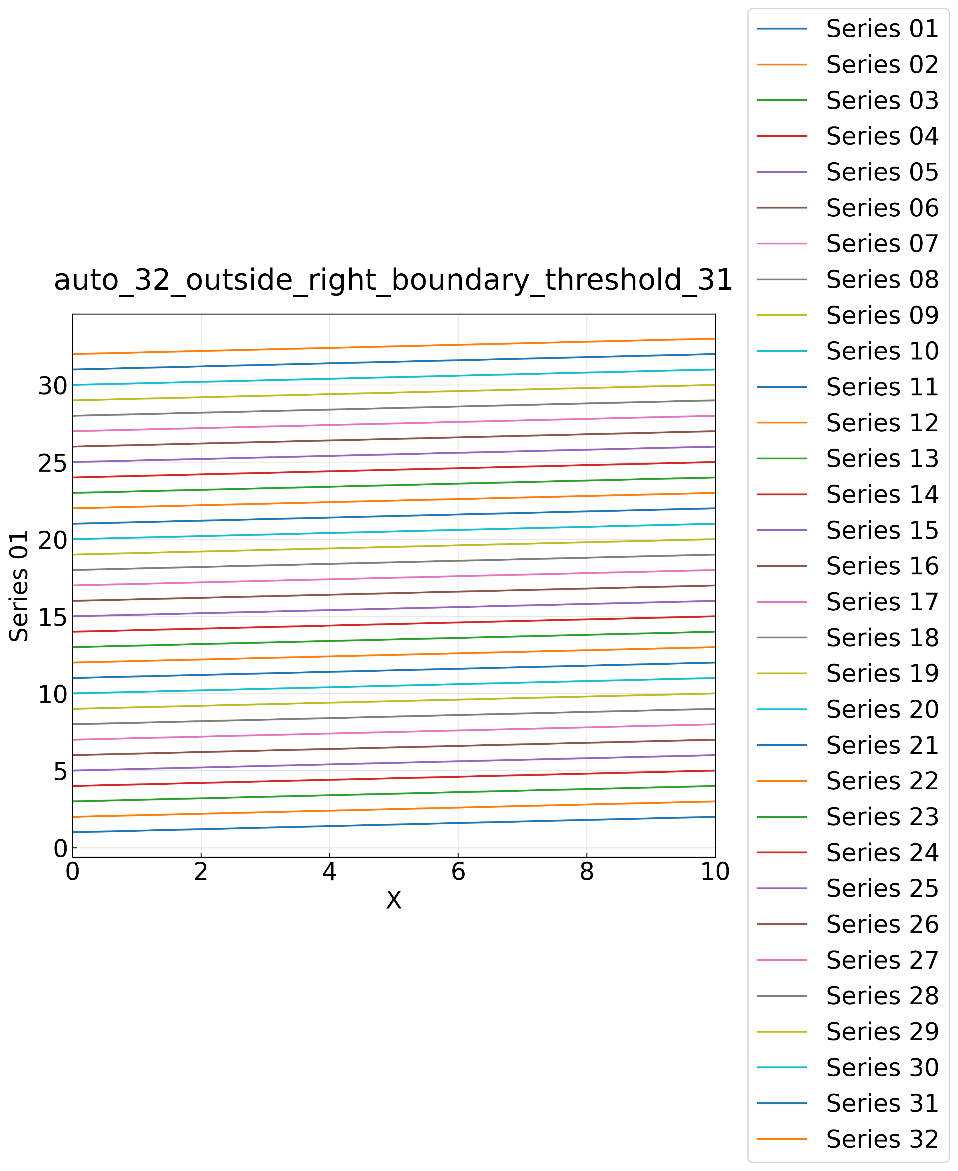
The switch to outside-right happens when the item count exceeds the threshold. With 32 series, threshold 32 keeps the legend inside while threshold 31 moves it outside (the bottom switch is disabled for this check).
The threshold-32 plot (legend kept inside) shows 32 items overflowing the plot area. It is included as a real example of why inside placement should not be used with many series.
1 2 3 4 5 6 7 8 9 10 11 12 13 14 15 16 17 | |
1 2 3 4 5 6 7 8 9 | |
Case 4: Boundary behavior of legend_bottom_threshold
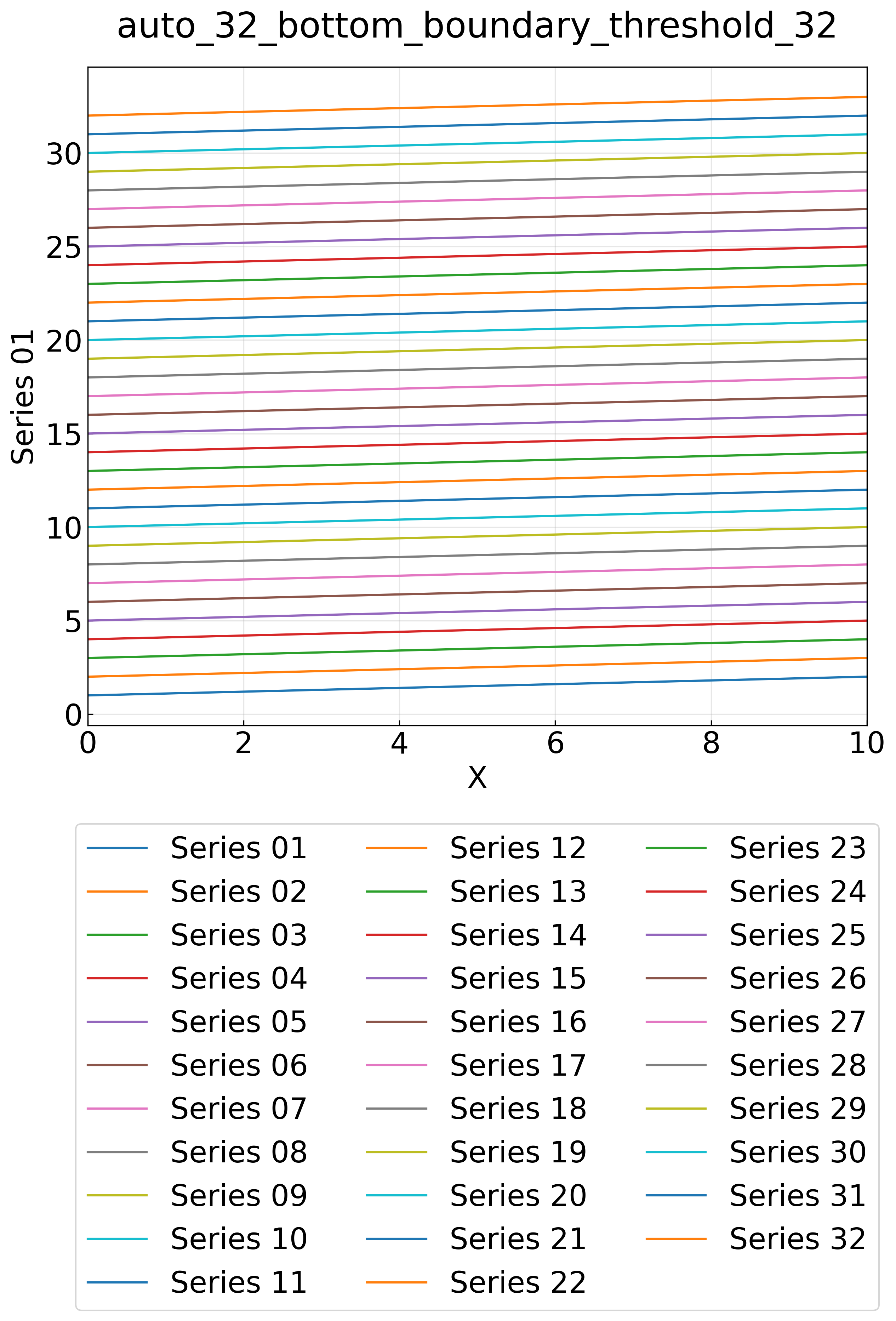
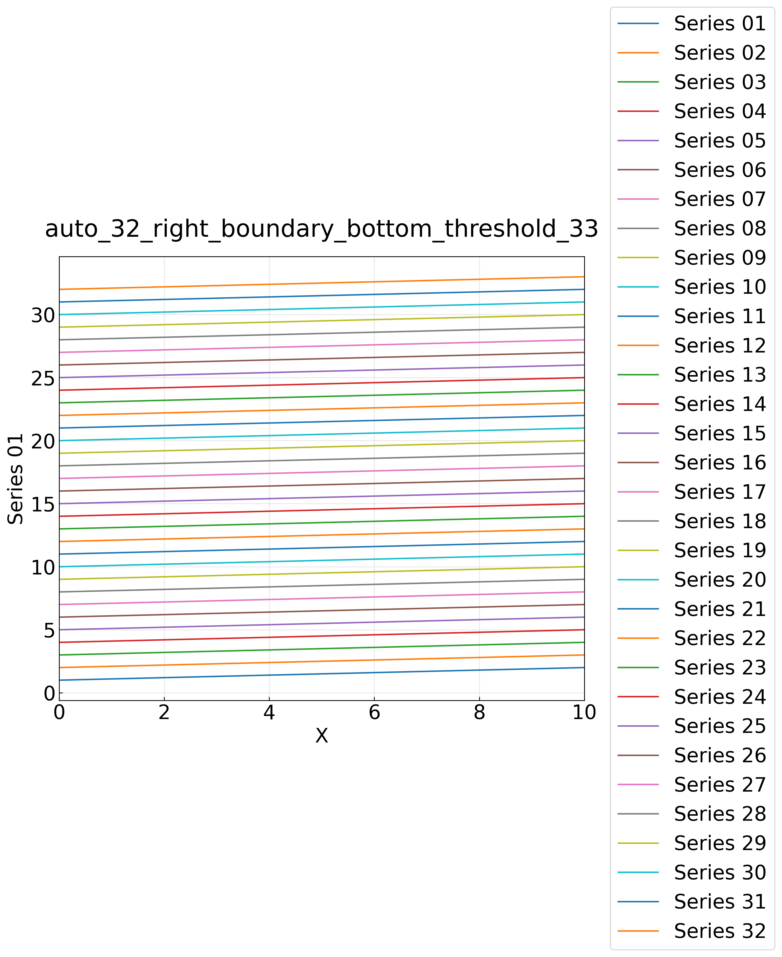
The switch to bottom placement happens at or above the threshold. With 32 series, threshold 32 places the legend below the graph while threshold 33 keeps it on the right.
1 2 3 4 5 6 7 8 9 10 11 12 13 14 15 16 17 | |
1 2 3 4 5 6 7 8 9 | |
Case 5: Forcing a placement (outside_right / outside_bottom)
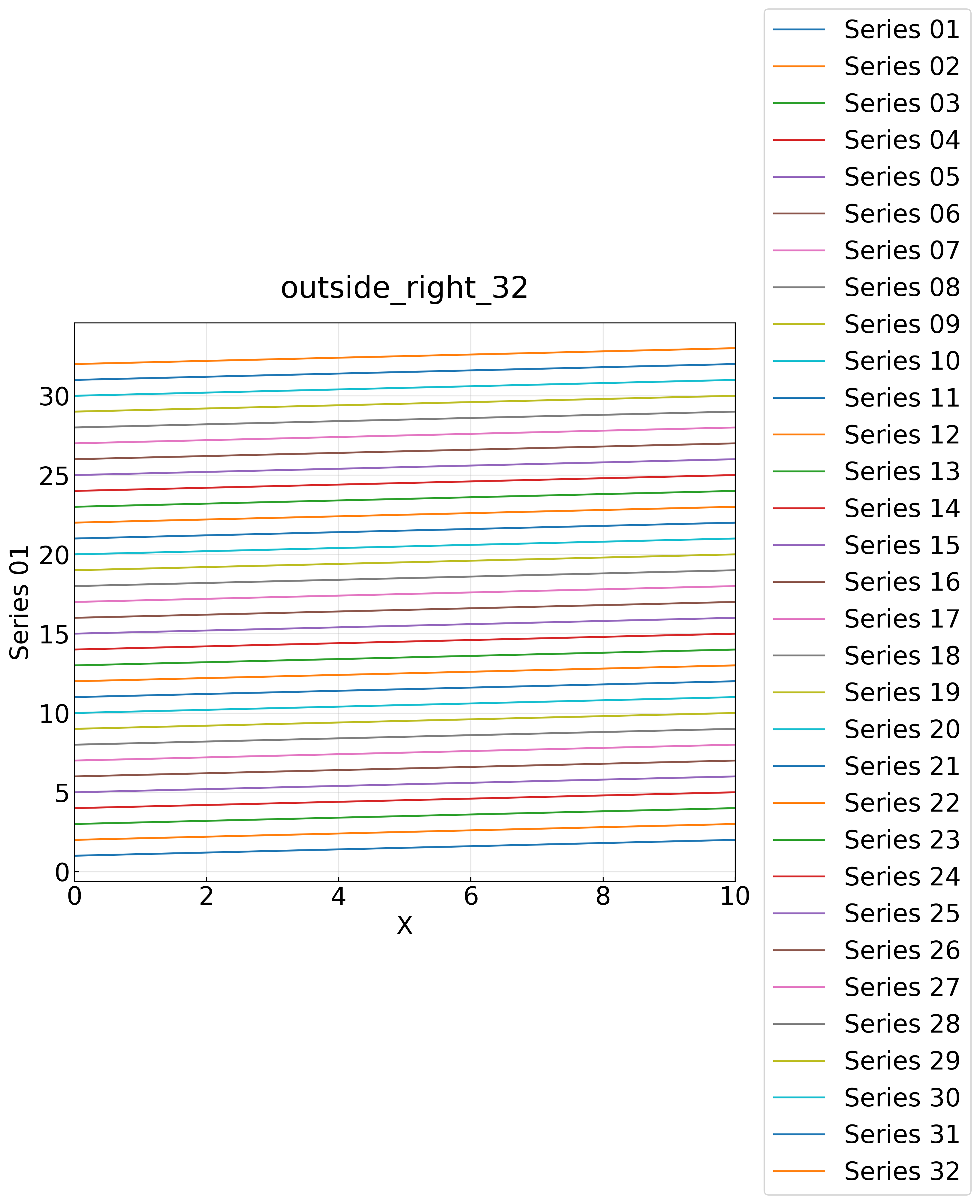
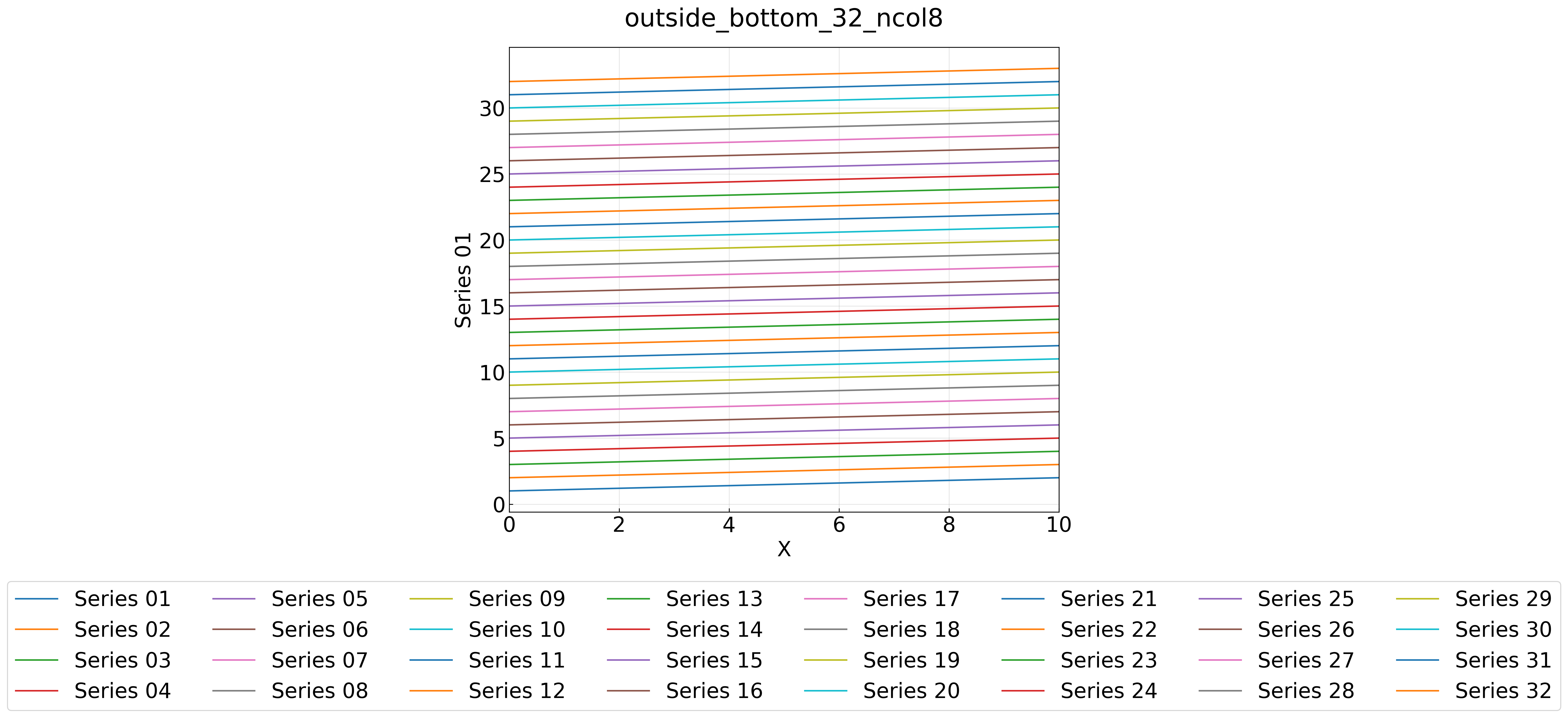
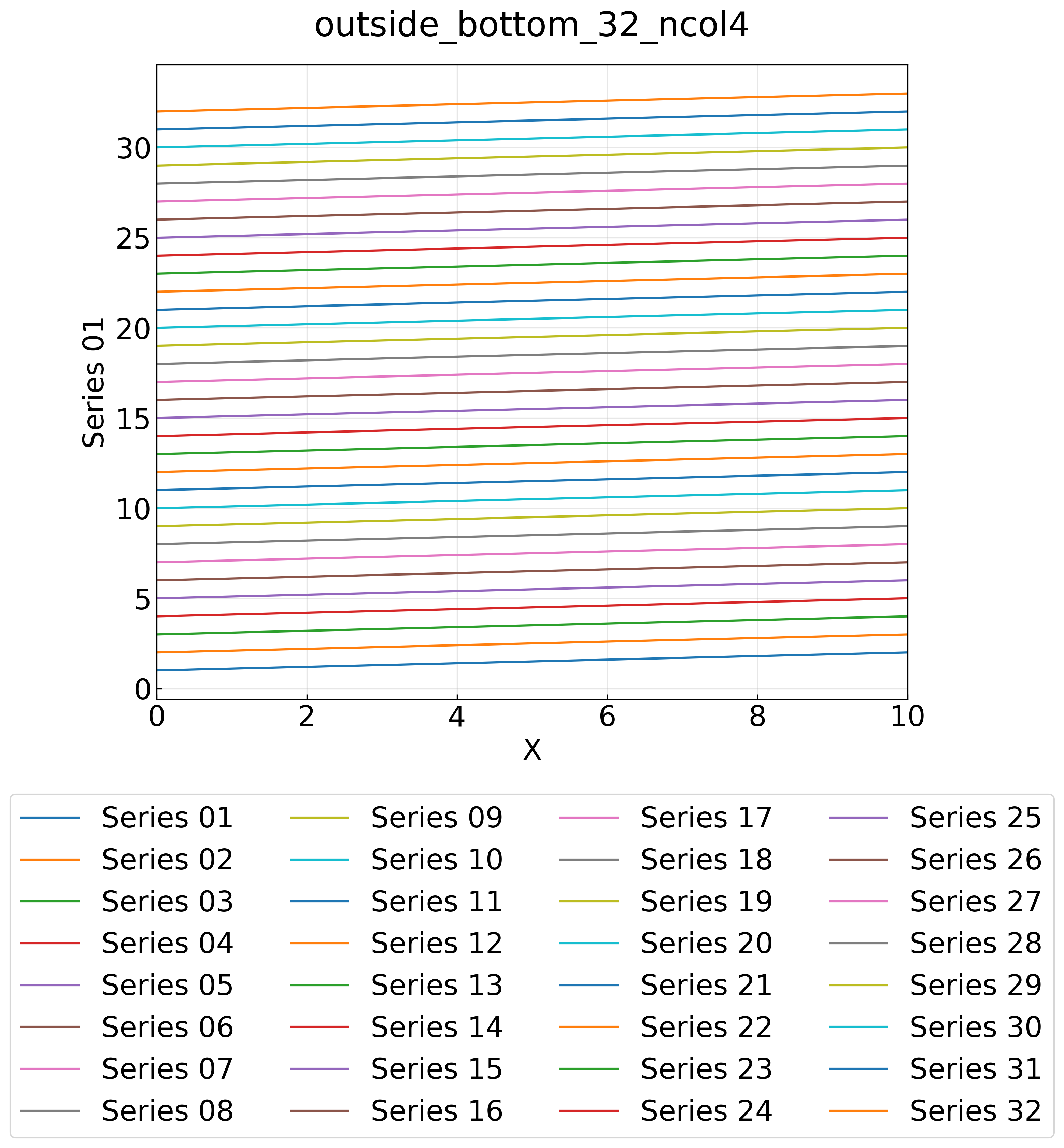
These examples pin the placement explicitly instead of using auto. With outside_bottom, legend_ncol controls the number of columns (and therefore rows).
1 2 3 4 5 6 7 8 9 10 11 12 13 14 15 | |
1 2 3 4 5 6 7 8 | |
Case 6: Hiding the legend (hide / exceeding max_legend_items)
An explicit hide, and an auto case where 32 series exceeds max_legend_items=30 so the legend is hidden automatically. The output images are equivalent.
1 2 3 4 5 6 7 8 9 10 11 12 13 14 | |
1 2 3 4 5 6 7 | |
Option Details
legend_bottom_threshold,--legend-bottom-threshold: Item-count threshold at whichautoswitches to bottom placement (default 21; switches at or above this value). PassNonein Python or0or less on the CLI to disable.legend_outside_threshold,--legend-outside-threshold: Threshold at whichautoswitches to outside-right placement (switches when exceeded). With the defaults (8 / 21): 1-8 items stay inside, 9-20 items go outside right, and 21+ items go below the graph.legend_ncol,--legend-ncol: Number of columns for bottom placement. The row count follows from items / columns (32 items x 8 columns = 4 rows).- With outside placements the canvas is enlarged while the plot area keeps its size, so the graph itself is never crushed no matter how many series there are.