コンテンツにスキップ

csv2graph サンプル集

csv2graph の主なオプションを実際のデータと合わせて確認できるサンプル集です。各セクションに記載されたコマンドは、サンプルのディレクトリ構成を再現するとそのまま実行できます。

各サンプルの CSV はこのページから直接ダウンロードできます。必要に応じて生成済み画像やスクリプトも合わせて公開しています。

サンプル1: オーバーレイのみ生成する基本例

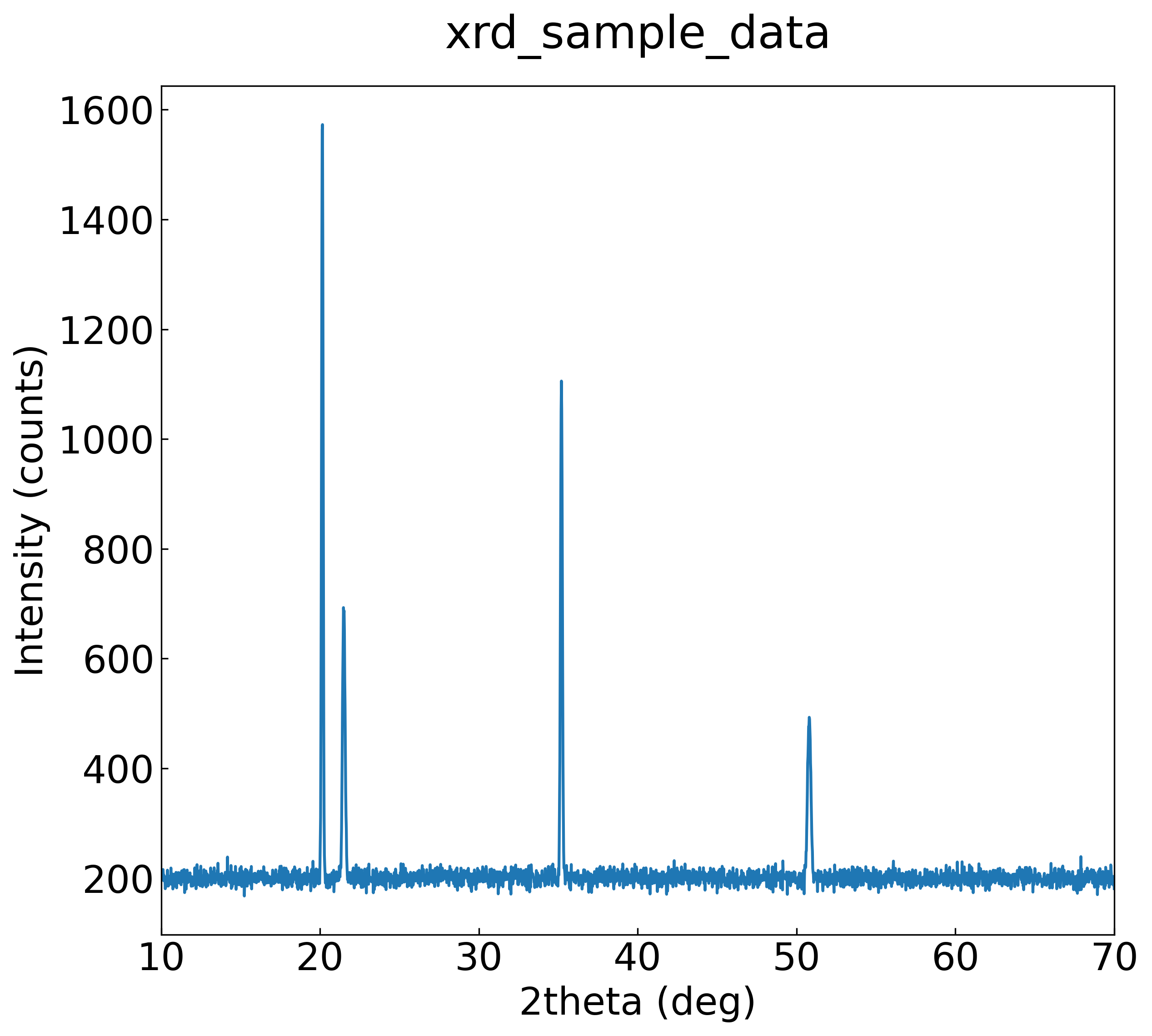
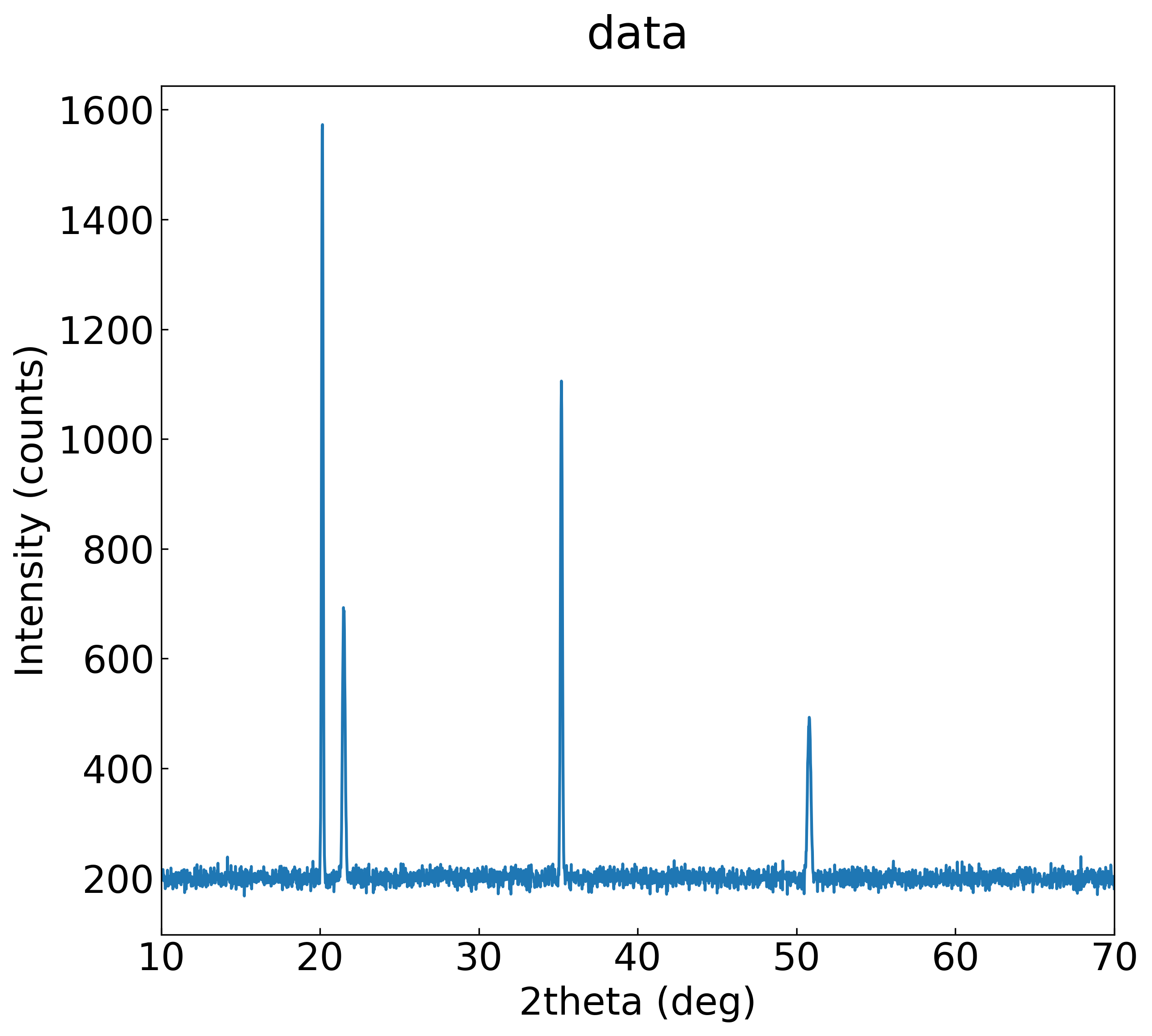
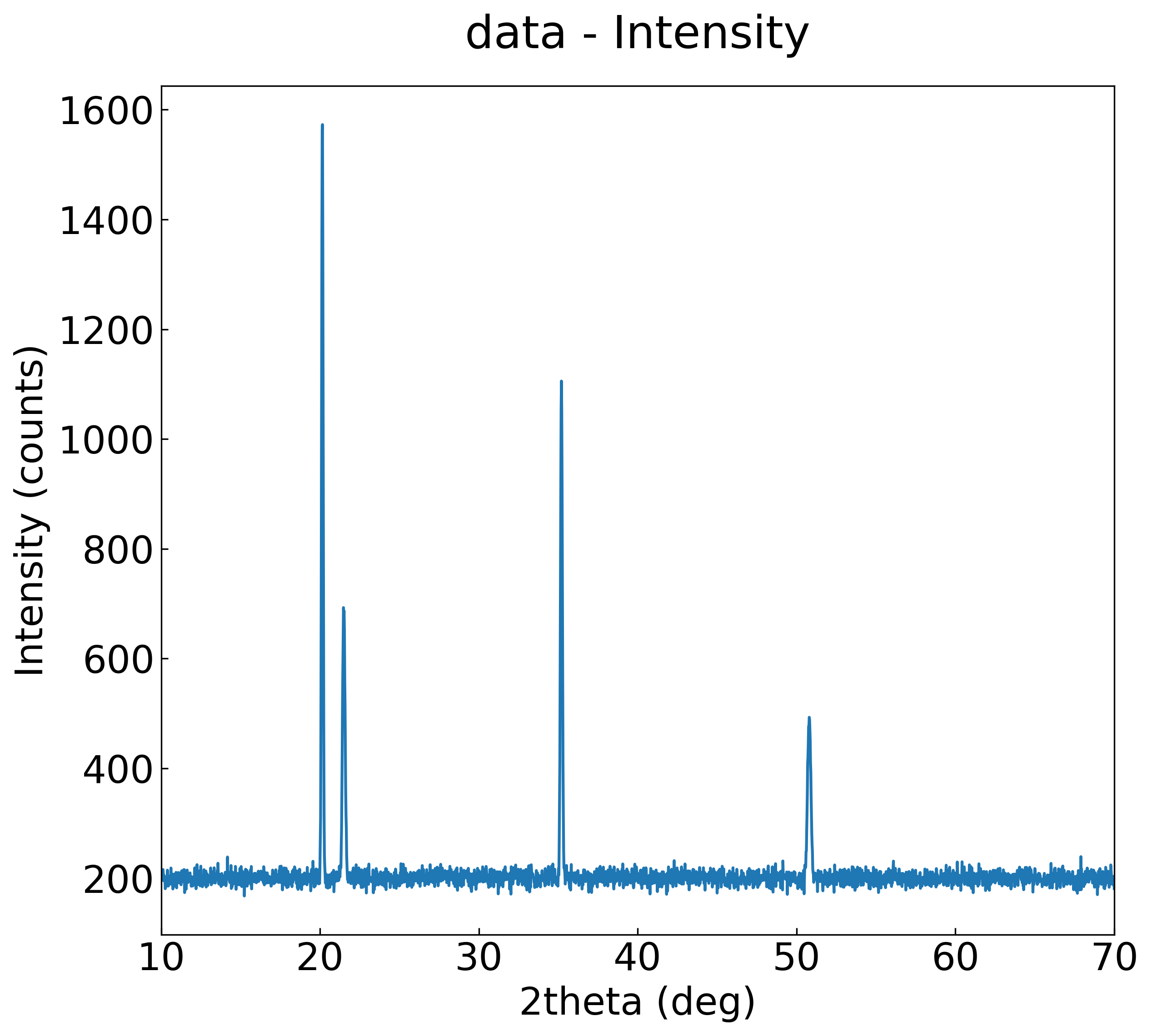
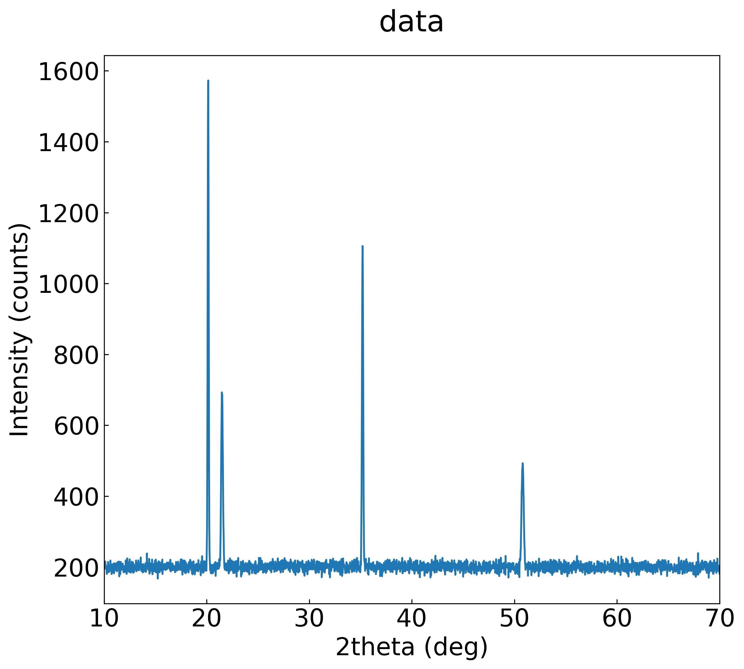
XRDのデータを使って --no-individual で代表グラフだけを出力する最小構成のサンプルです(単一系列でも個別画像を強制したい場合は --individual を指定してください)。

データの概要

以下のデータを使用します。XRDのデータを想定しています。

 1
 2
 3
 4
 5
 6
 7
 8
 9
10
2theta (deg),Intensity (counts)
10.0,204.9671
10.02,198.6174
10.04,206.4769
10.06,215.2303
10.08,197.6585
10.1,197.6586
10.12,215.7921
10.14,207.6743
...

Overlay: xrd_sample

ディレクトリ構造

1
2
3
4
sample1/
├── data.csv
├── data.png
└── sample.py

実行例

以下のタブで Python と CLI の実行例を切り替えられます。

 1
 2
 3
 4
 5
 6
 7
 8
 9
10
#sample.py
from pathlib import Path

from rdetoolkit.graph import csv2graph

if __name__ == "__main__":
    csv2graph(
        csv_path=Path("sample1/data.csv"),
        no_individual=True,  # --no-individual
    )
1
rdetoolkit csv2graph 'sample1/data.csv' --no-individual

オプションの説明

  • no_individual=True, --no-individual : 個別グラフは作らずオーバーレイ画像だけを作成します。

サンプル2: Y 軸を対数表示する

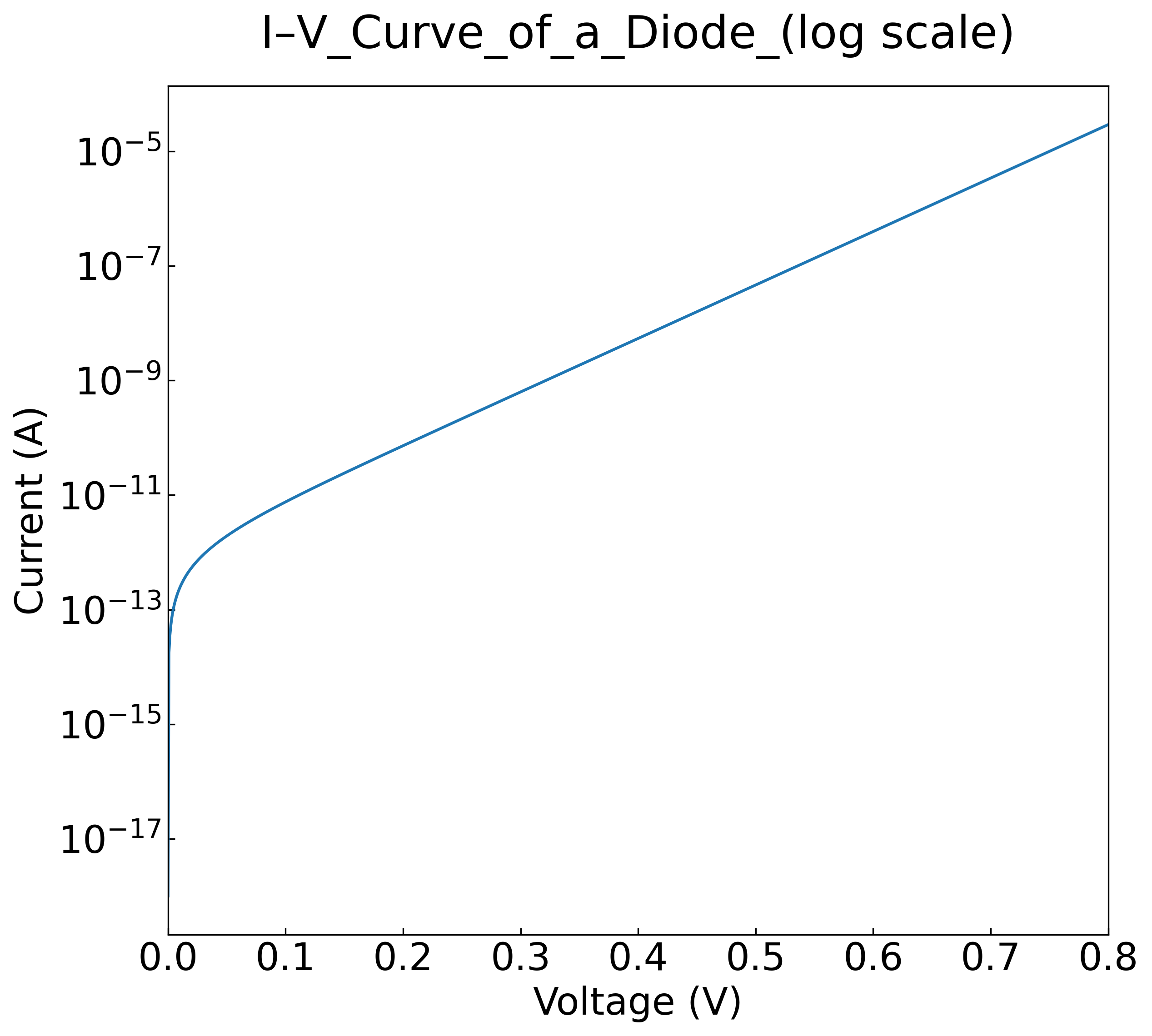
XRD 想定データを --logy で対数スケール表示し、タイトルを指定するサンプルです。

データの概要

以下のデータを使用します。ダイオードのI–V特性のデータを想定しています。

1
2
3
4
5
Voltage (V),Current (A)
0.0,9.999999999999999e-19
0.0008008008008008008,1.735937164947776e-14
0.0016016016016016017,3.5020091083020285e-14
...

Overlay

ディレクトリ構造

1
2
3
sample2/
├── data.csv
└── sample_log_scale.py

実行例

以下のタブで Python と CLI の実行例を切り替えられます。

 1
 2
 3
 4
 5
 6
 7
 8
 9
10
11
# sample_log_scale.py
from pathlib import Path

from rdetoolkit.graph import csv2graph

if __name__ == "__main__":
    csv2graph(
        csv_path=Path("sample2/data.csv"),
        logy=True,
        title="I–V_Curve_of_a_Diode_(log scale)",
    )
1
2
3
4
rdetoolkit csv2graph sample2/data.csv \
  --logy \
  --no-individual \
  --title "I–V_Curve_of_a_Diode_(log scale)"

オプションの説明

  • no_individual=True, --no-individual : 個別グラフは作らずオーバーレイ画像だけを作成します。
  • --logy / logy=True: Y 軸を対数スケールで描画します。

今回はサンプルとして存在しませんが、X軸を対数スケールで描画する時は、--logx / logx=Trueを使用します。

サンプル3: 軸反転(X/Y)

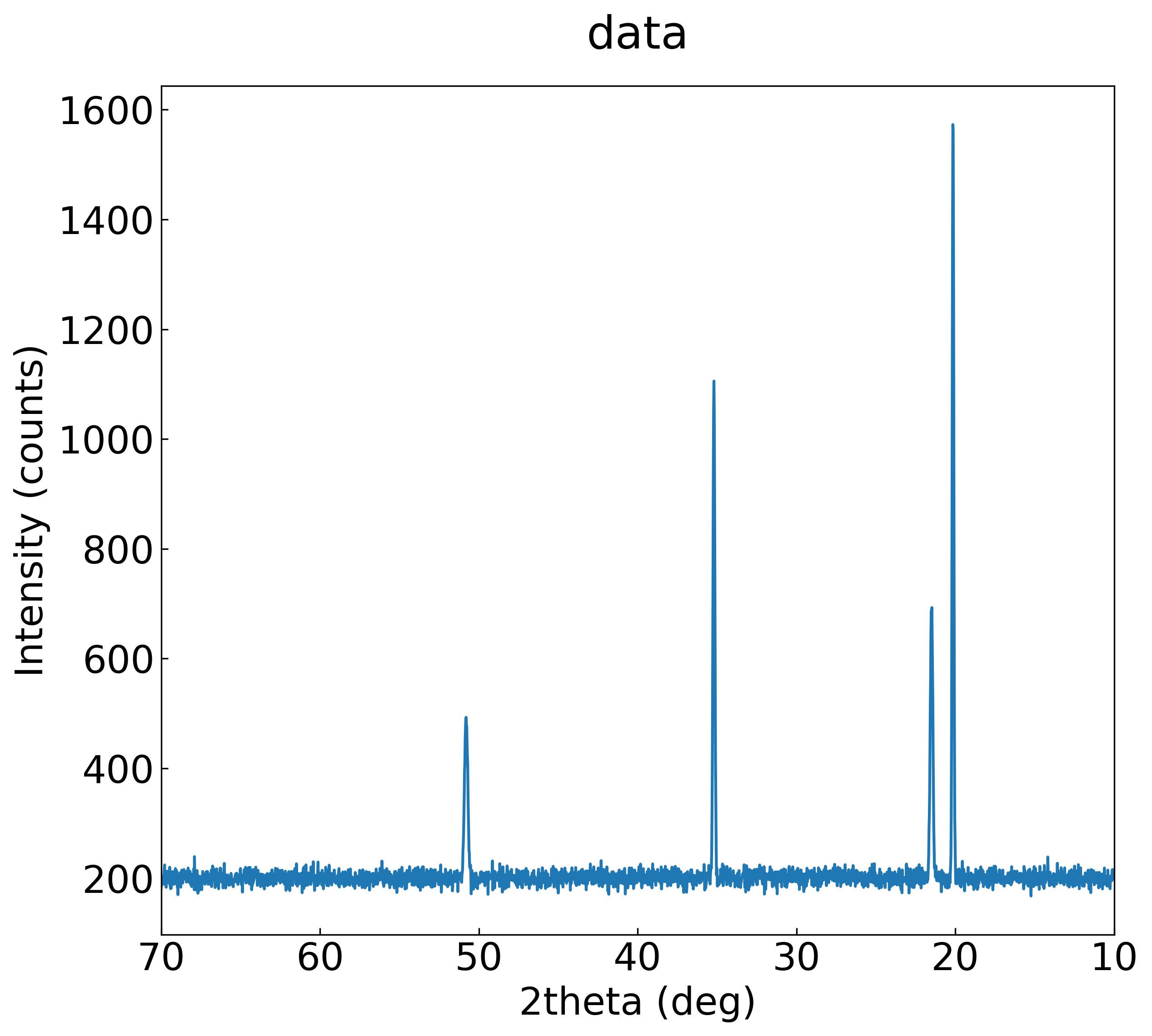
XRD データを使い、--invert-x--invert-y で軸を反転する使い方をまとめています。

データの概要

以下のデータを使用します。XRDのデータを想定しています。

 1
 2
 3
 4
 5
 6
 7
 8
 9
10
2theta (deg),Intensity (counts)
10.0,204.9671
10.02,198.6174
10.04,206.4769
10.06,215.2303
10.08,197.6585
10.1,197.6586
10.12,215.7921
10.14,207.6743
...

Overlay

ディレクトリ構成

実行前のディレクトリ構成

1
2
3
sample3/
├── data.csv
└── sample_invert.py

X軸を反転させる例

以下のタブで Python と CLI の実行例を切り替えられます。

 1
 2
 3
 4
 5
 6
 7
 8
 9
10
11
12
# sample_invert.py
from pathlib import Path

from rdetoolkit.graph import csv2graph

if __name__ == "__main__":
    # invert_x
    csv2graph(
        csv_path=Path("sample3/data.csv"),
        invert_x=True,  # --invert-x
        no_individual=True,  # --no-individual
    )
1
rdetoolkit csv2graph 'sample3/data.csv' --invert-x --no-individual

Y軸を反転させる例

 1
 2
 3
 4
 5
 6
 7
 8
 9
10
11
# sample_invert.py
from pathlib import Path
from rdetoolkit.graph import csv2graph

if __name__ == "__main__":
    # invert_y
    csv2graph(
        csv_path=Path("sample3/data.csv"),
        invert_y=True,  # --invert-y
        no_individual=True,
    )
1
rdetoolkit csv2graph 'sample3/data.csv' --invert-y --no-individual

オプションの説明

  • invert_x=True, --invert-x : 出力画像の X 軸は左右反転します。
  • invert_y=True, --invert-y : 出力画像の Y 軸は上下反転します。
  • no_individual=True : 個別グラフは作らずオーバーレイ画像だけを作成します。

サンプル4: 複数ペアの系列をオーバーレイ

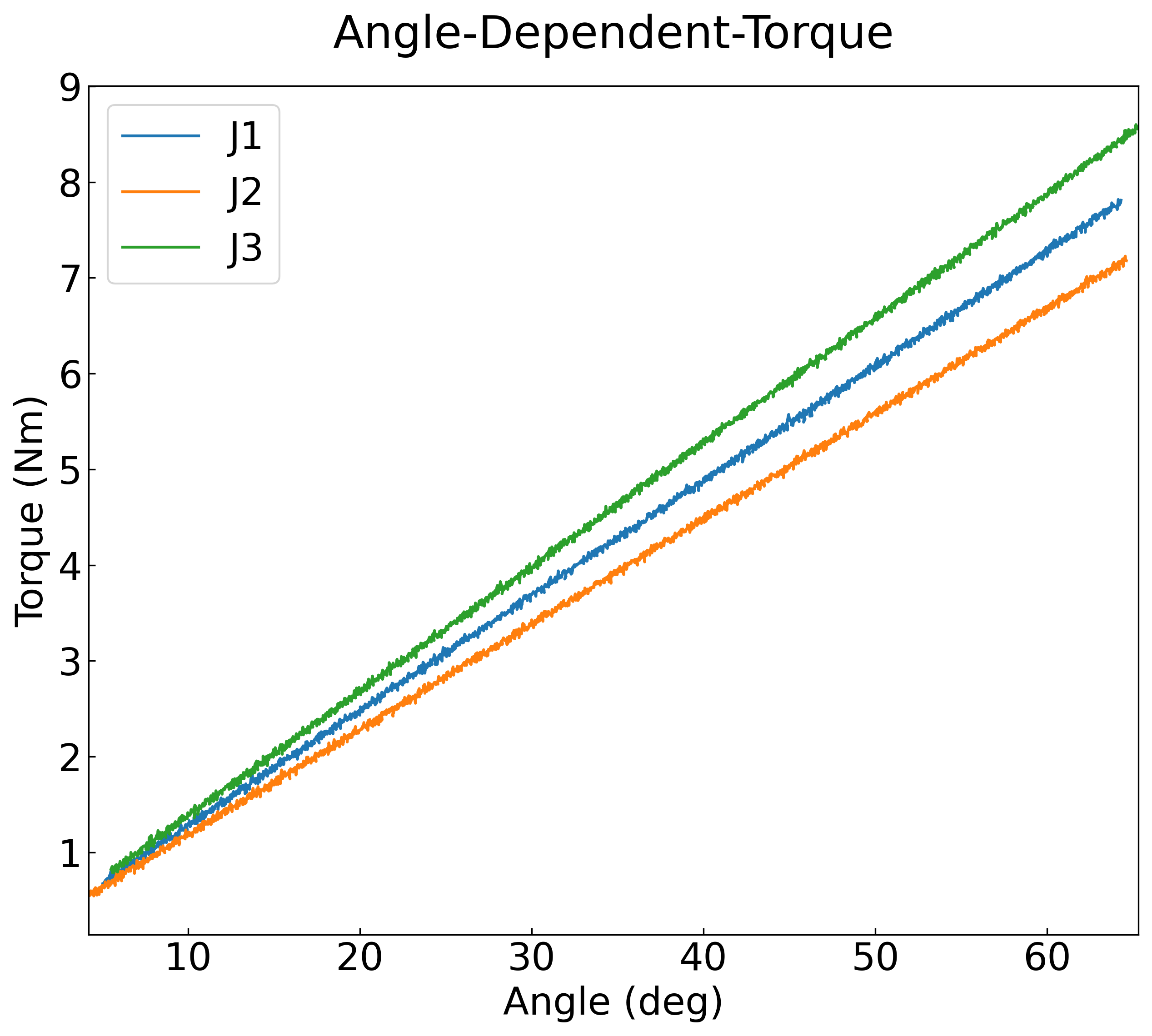
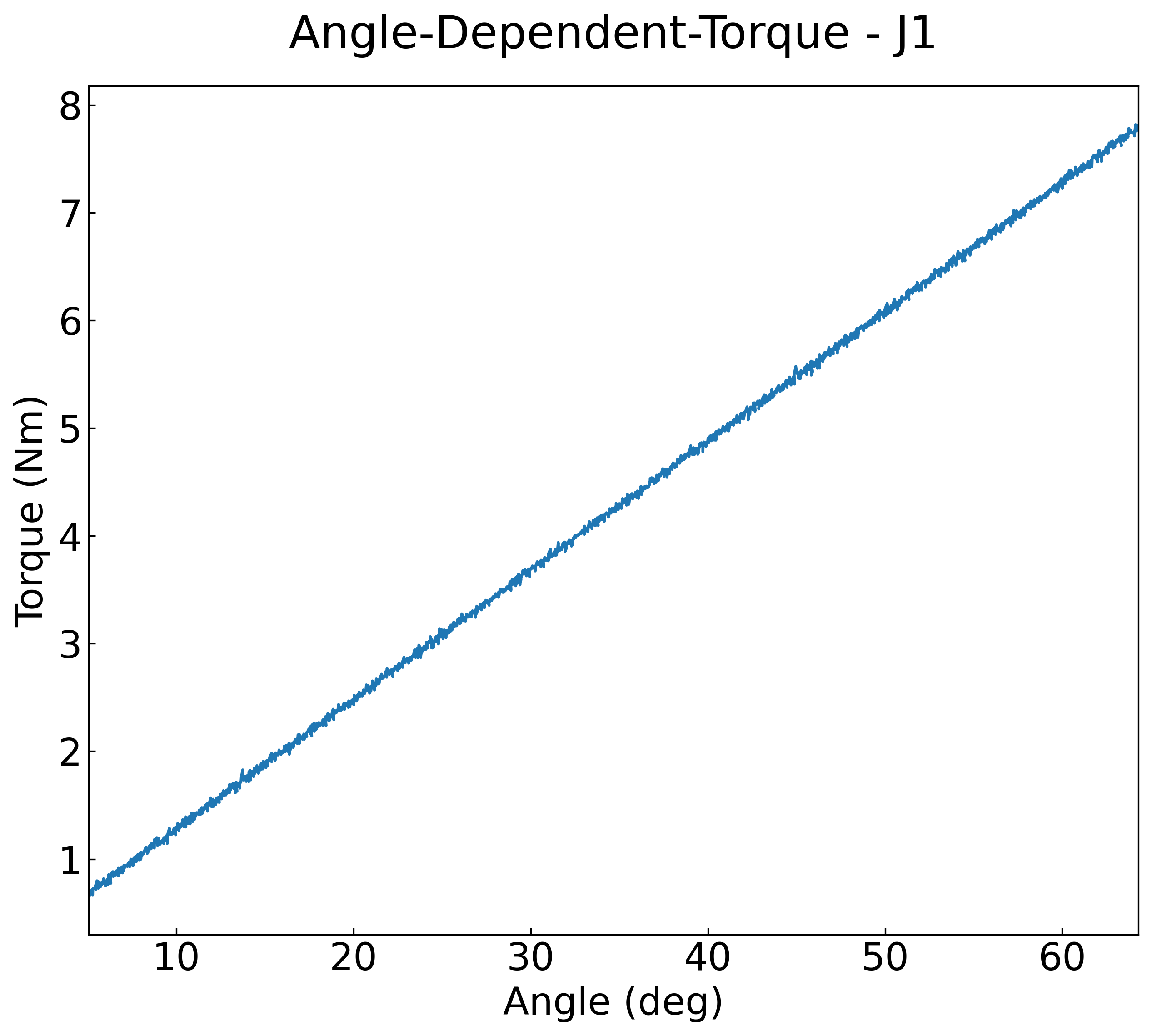
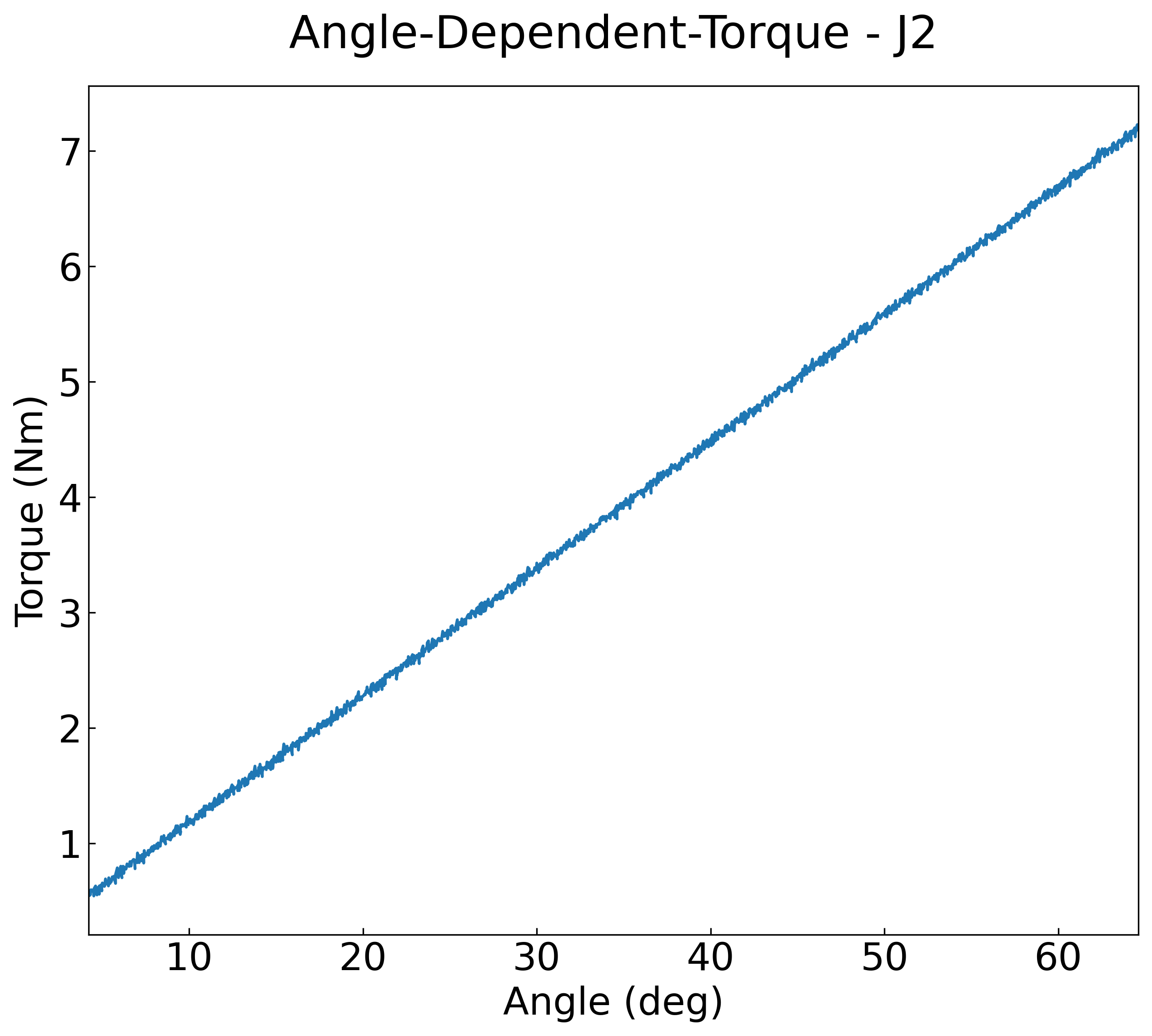
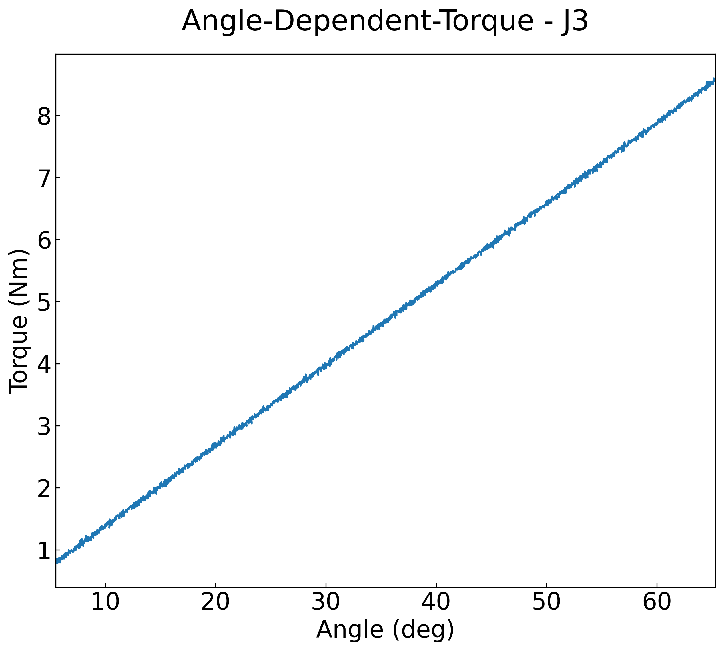
3 関節トルクのデータを複数ペアの X/Y 列で描画し、オーバーレイと個別グラフをまとめて出力します。

データの概要

以下のデータを使用します。3関節(J1–J3)の角度・角速度・トルクを、ほぼ単調増加の角度と線形モデル+微小ノイズで生成した合成時系列データです。

1
2
3
4
5
6
Phase-U:volt(V),Phase-U:curr(A),Phase-U:power(kW),Phase-V:volt(V),Phase-V:curr(A),Phase-V:power(kW),Phase-W:volt(V),Phase-W:curr(A),Phase-W:power(kW)
230.1,10.02,2.126,231.0,10.11,2.116,229.7,10.15,2.13
230.1,9.94,2.109,231.1,10.26,2.138,229.8,10.06,2.118
230.2,9.83,2.077,231.0,10.09,2.096,229.3,10.05,2.075
230.4,10.14,2.161,231.0,10.27,2.135,229.4,10.27,2.176
...

Overlay: 3 Joint Torque vs Angle

J1 Torque vs Angle

J2 Torque vs Angle

J3 Torque vs Angle

ディレクトリ構成

実行前のディレクトリ構成

1
2
3
sample4/
├── data.csv
└── sample_pair_plot.py

実行例

以下のタブで Python と CLI の実行例を切り替えられます。

 1
 2
 3
 4
 5
 6
 7
 8
 9
10
11
12
13
# sample_pair_plot.py
from pathlib import Path

from rdetoolkit.graph import csv2graph

if __name__ == "__main__":
    csv2graph(
        csv_path=Path("sample4/data.csv"),
        mode="overlay",
        x_col=[1, 4, 7],
        y_cols=[0, 3, 6],
        title="Angle-Dependent-Torque",
    )
1
2
3
4
5
rdetoolkit csv2graph sample4/data.csv \
    --mode overlay \
    --x-col 1 --x-col 4 --x-col 7 \
    --y-cols 0 --y-cols 3 --y-cols 6 \
    --title "Angle-Dependent-Torque"

オプションの説明

  • --mode overlay: 全系列を1枚のグラフに重ねるモード(x1y1x2y2 相当)を選択します。
  • --x-col 1 --x-col 4 --x-col 7: X 軸に使う列を3つ指定します(0始まりで 2 列目、5 列目、8 列目)。以下のy列と順番にペアリングされます。
  • --y-cols 0 --y-cols 3 --y-cols 6: Y 軸に使う列を3つ指定します(1 列目、4 列目、7 列目)。それぞれx列とペアになり、3本の系列として描画されます。
  • --title "Angle-Dependent Torque": 生成されるグラフのタイトルと出力ファイル名の基礎名を "Angle-Dependent Torque" に設定します。

サンプル5: 単一の X 列と複数 Y 系列

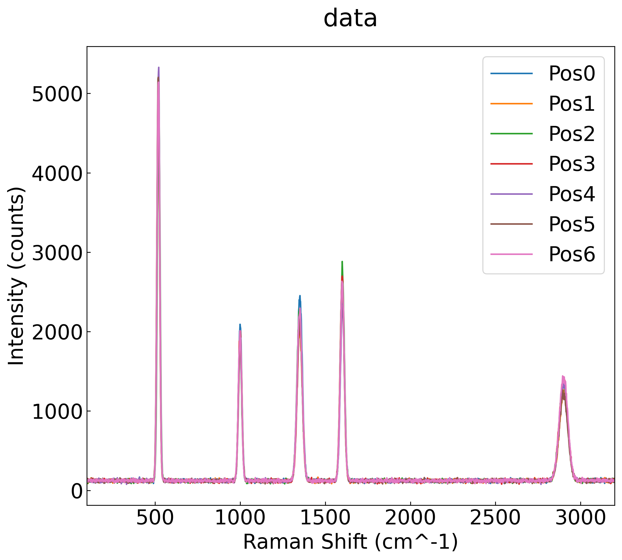
ラマン分光データで 1 本の X 列と複数 Y 系列を組み合わせ、タイトルを変更する例です。

データの概要

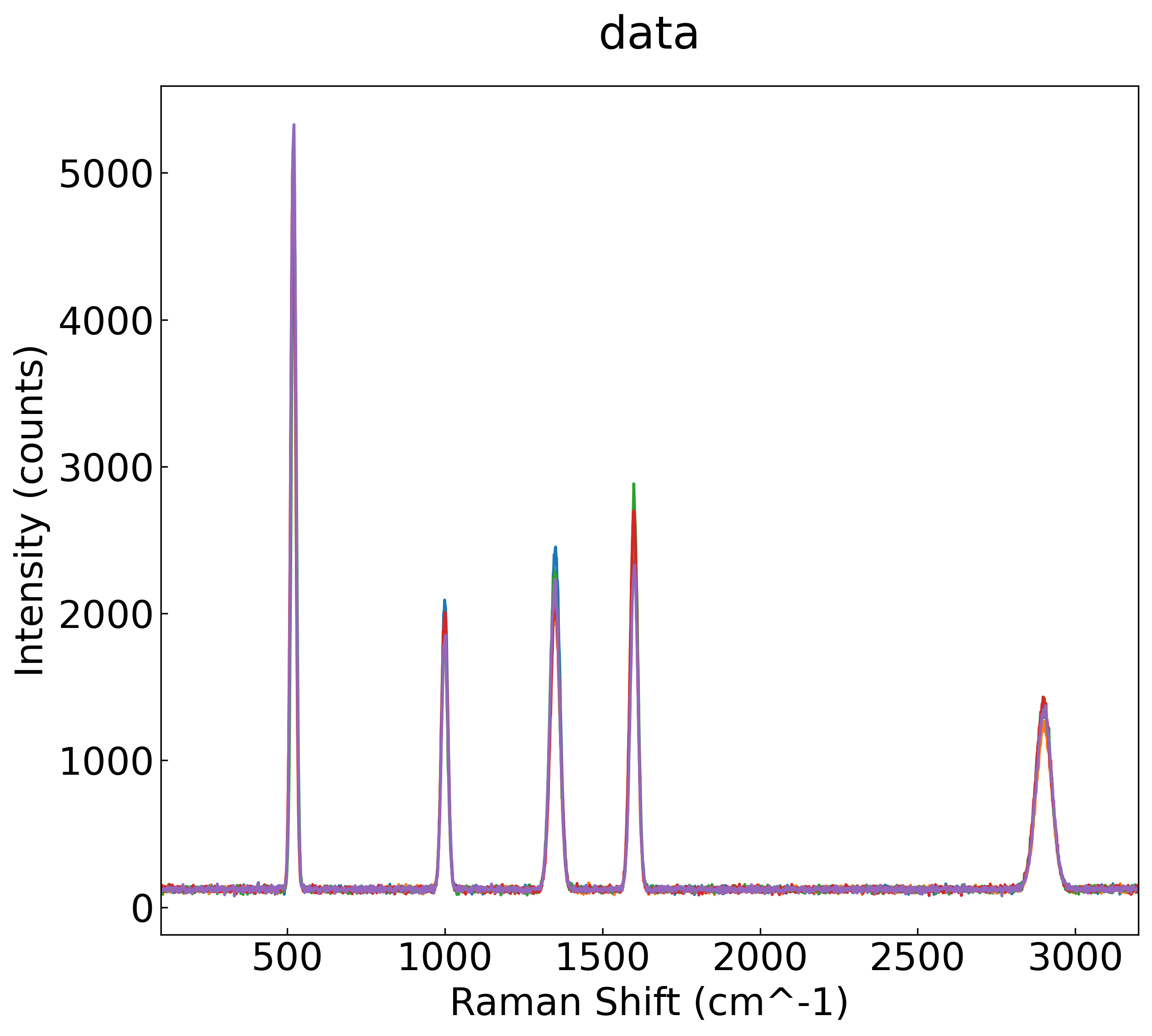
以下のデータを使用します。ラマン分光のダミーデータを想定しています。横軸 Raman Shift (cm⁻¹) に対して、Pos0~Pos10 の各測定位置での Intensity (counts)(スペクトル強度)を並べています。

1
2
3
4
5
6
7
Raman Shift (cm^-1),Pos0: Intensity (counts),Pos1: Intensity (counts),Pos2: Intensity (counts),Pos3: Intensity (counts),Pos4: Intensity (counts),Pos5: Intensity (counts),Pos6: Intensity (counts),Pos7: Intensity (counts),Pos8: Intensity (counts),Pos9: Intensity (counts),Average: Intensity (counts)
100.0,117.0,124.0,134.0,135.0,111.0,126.0,132.0,116.0,126.0,114.0,124.0
101.551,117.0,126.0,106.0,138.0,110.0,127.0,134.0,146.0,134.0,116.0,125.0
103.102,126.0,139.0,110.0,150.0,119.0,134.0,128.0,128.0,116.0,141.0,129.0
104.652,100.0,108.0,90.0,119.0,118.0,145.0,106.0,117.0,144.0,117.0,116.0
106.203,102.0,87.0,114.0,125.0,117.0,108.0,112.0,117.0,133.0,136.0,115.0
...

Overlay: raman

ディレクトリ構成

実行前のディレクトリ構成

1
2
3
sample5/
├── data.csv
└── sample_custom_title.py

実行例

以下のタブで Python と CLI の実行例を切り替えられます。

 1
 2
 3
 4
 5
 6
 7
 8
 9
10
11
12
13
# sample_custom_title.py
from pathlib import Path

from rdetoolkit.graph import csv2graph

if __name__ == "__main__":
    csv2graph(
        csv_path=Path("sample5/data.csv"),
        mode="overlay",
        x_col=[1, 4, 7],
        y_cols=[0, 3, 6],
        title="Angle-Dependent-Torque",
    )
1
2
3
4
5
rdetoolkit csv2graph sample5/data.csv \
  --x-col 0 \
  --y-cols 1 --y-cols 2 --y-cols 3 --y-cols 4 --y-cols 5 \
  --no-individual
  --title "Angle-Dependent-Torque"

オプションの説明

  • --x-col 0:X 軸用の列。ひとつ指定すれば、後続の Y 列すべてと自動でペアリングされます。
  • --y-cols 1 … 5:描画したい Y 系列(5 列)を 0 始まりで列番号指定。
  • --no-individual:統合プロットだけを出力。個別 PNG の生成を抑止します。
  • --title: カスタムグラフタイトル

サンプル6: 凡例表示件数を制限

ラマン分光データで --max-legend-items により凡例の表示件数を抑えるサンプルです。

データの概要

以下のデータを使用します。ラマン分光のダミーデータを想定しています。横軸 Raman Shift (cm⁻¹) に対して、Pos0~Pos10 の各測定位置での Intensity (counts)(スペクトル強度)を並べています。

1
2
3
4
5
6
7
Raman Shift (cm^-1),Pos0: Intensity (counts),Pos1: Intensity (counts),Pos2: Intensity (counts),Pos3: Intensity (counts),Pos4: Intensity (counts),Pos5: Intensity (counts),Pos6: Intensity (counts),Pos7: Intensity (counts),Pos8: Intensity (counts),Pos9: Intensity (counts),Average: Intensity (counts)
100.0,117.0,124.0,134.0,135.0,111.0,126.0,132.0,116.0,126.0,114.0,124.0
101.551,117.0,126.0,106.0,138.0,110.0,127.0,134.0,146.0,134.0,116.0,125.0
103.102,126.0,139.0,110.0,150.0,119.0,134.0,128.0,128.0,116.0,141.0,129.0
104.652,100.0,108.0,90.0,119.0,118.0,145.0,106.0,117.0,144.0,117.0,116.0
106.203,102.0,87.0,114.0,125.0,117.0,108.0,112.0,117.0,133.0,136.0,115.0
...

Overlay: raman_max_legend_items

ディレクトリ構成

実行前のディレクトリ構成

1
2
3
sample6/
├── data.csv
└── sample_max_legend_items.py

実行例

以下のタブで Python と CLI の実行例を切り替えられます。

 1
 2
 3
 4
 5
 6
 7
 8
 9
10
11
12
13
# sample_max_legend_items.py
from pathlib import Path

from rdetoolkit.graph import csv2graph

if __name__ == "__main__":
    csv2graph(
        "sample6/data.csv",
        x_col=0,
        y_cols=[1, 2, 3, 4, 5],
        no_individual=True,
        max_legend_items=3,
    )
1
2
3
4
5
rdetoolkit csv2graph sample6/data.csv \
  --x-col 0 \
  --y-cols 1 --y-cols 2 --y-cols 3 --y-cols 4 --y-cols 5 \
  --no-individual \
  --max-legend-items 3

オプションの説明

  • --x-col 0 は X 軸に 0 列目を使う指定。1 度だけ書けば後続のすべての Y 列と自動でペアになります。
  • --y-cols … で 1〜5 列目の 5 系列を指定します。
  • --no-individual で統合プロットの PNG のみ生成し、個別 PNG をスキップします。
  • --max-legend-items 3 で凡例の表示件数を 3 件までに制限します(超えると凡例が非表示になります)。

サンプル7: 多チャンネル充放電データのオーバーレイ

充放電状態ラベルを複数列で扱い、方向列ごとに系列を色分けしながら --output-dir を切り替える高度な例です。

サンプルには生成済み画像を含めていないため、出力例を得るにはコードを実行してください。

データの概要

以下のデータを使用します。充放電特性のダミーデータを想定しています。

1
2
3
4
state_ch1,time_ch1[s],step_index_ch1,current_ch1[A],capacity_ch1[mAh],voltage_ch1[V],state_ch2,time_ch2[s],step_index_ch2,current_ch2[A],capacity_ch2[mAh],voltage_ch2[V],state_ch3,time_ch3[s],step_index_ch3,current_ch3[A],capacity_ch3[mAh],voltage_ch3[V],state_ch4,time_ch4[s],step_index_ch4,current_ch4[A],capacity_ch4[mAh],voltage_ch4[V],state_ch5,time_ch5[s],step_index_ch5,current_ch5[A],capacity_ch5[mAh],voltage_ch5[V],state_ch6,time_ch6[s],step_index_ch6,current_ch6[A],capacity_ch6[mAh],voltage_ch6[V]
Charge,0.0,1,1.0248357076505616,0.0,3.1464269673816196,Discharge,0.0,1,-0.9246489863932321,0.0,3.26398992423171,Discharge,0.0,1,-0.9703987550711959,0.0,3.301646178292083,Discharge,0.0,1,-0.8373920481516945,0.0,3.2405780651132403,Discharge,0.0,1,-1.0452295606856536,0.0,3.289520156004168,Discharge,0.0,1,-1.1267131011336096,0.0,3.2782242976855556
Charge,2.0,1,0.9930867849414408,0.5693531709169787,3.1401720080365,Discharge,2.0,1,-0.9528697682537017,0.0,3.2612743372332664,Discharge,2.0,1,-1.079386898465995,0.0,3.3142719992060634,Discharge,2.0,1,-0.9061484473317185,0.0,3.2529616227280664,Discharge,2.0,1,-0.9533585647953902,0.0,3.2768224979535368,Discharge,2.0,1,-1.0899924167596289,0.0,3.27788892249149
...

実行例

以下のタブで Python と CLI の実行例を切り替えられます。

 1
 2
 3
 4
 5
 6
 7
 8
 9
10
11
12
13
14
from pathlib import Path

from rdetoolkit.graph import csv2graph

if __name__ == "__main__":
    csv2graph(
        Path("sample7/data.csv"),
        x_col=[1, 7, 13, 19, 25, 31],
        y_cols=[5, 11, 17, 23, 29, 35],
        direction_cols=[0, 6, 12, 18, 24, 30],
        max_legend_items=5,
        title="Charge_Rest_Discharge",
        output_dir=Path("./custom_output"),
    )
1
2
3
4
5
6
7
8
rdetoolkit csv2graph sample7/data.csv \
  --x-col 1 --x-col 7 --x-col 13 --x-col 19 --x-col 25 --x-col 31 \
  --y-cols 5 --y-cols 11 --y-cols 17 --y-cols 23 --y-cols 29 --y-cols 35 \
  --direction-cols 0 --direction-cols 6 --direction-cols 12 \
  --direction-cols 18 --direction-cols 24 --direction-cols 30 \
  --logx --logy --max-legend-items 5 \
  --title "Charge_Rest_Discharge" \
  --output-dir ./custom_output

オプションの説明

  • --output-dir ./custom_output
  • 生成した PNG/HTML を保存するディレクトリ。指定がないと入力 CSV と同じフォルダになりますが、ここでは ./output にまとめて出力します。
  • --title "Charge_Rest_Discharge"
  • グラフのタイトルと、出力ファイル名のベース("Charge_Rest_Discharge.png など)を設定します。
  • --mode overlay
  • すべての系列を 1 枚に重ね描きするモード。旧 CLI の x1y1x2y2 と同じで、複数の X/Y 列を一対一にペアリングします。
  • --x-col 1 --x-col 7 … 43
  • 横軸に使う列番号を列挙します(0 始まり)。ここでは 8 本の系列があり、列 1,7,13,…,43 がそれぞれの X 軸として使われます。CLI ではオプションを列数ぶん繰り返して 指定します。
  • --y-cols 5 --y-cols 11 … 47
  • 縦軸に使う列番号。X と同じ順番で 8 本指定し、列 5,11,17,…,47 を Y 系列として描画します。x_col と y_cols は位置対応でペアになります。
  • --direction-cols 0, --direction-cols 6 … 42
  • 各 Y 系列に対応する「方向」列を指定します。列 0,6,12,…,42 には例えば Charge / Discharge などの状態ラベルが入っている想定で、その値ごとに線色を変えたり、セグ メントを分けたりします。系列ごとに違う方向列を指定したい場合は、Y 系列と同じ回数このオプションを繰り返します。
  • --max-legend-items 5
  • 凡例に表示する項目数の上限。方向や系列が多い場合、6 件目以降の凡例を自動的に非表示にしてプロットを読みやすくします。

サンプル8: 凡例の横に補足情報を表示

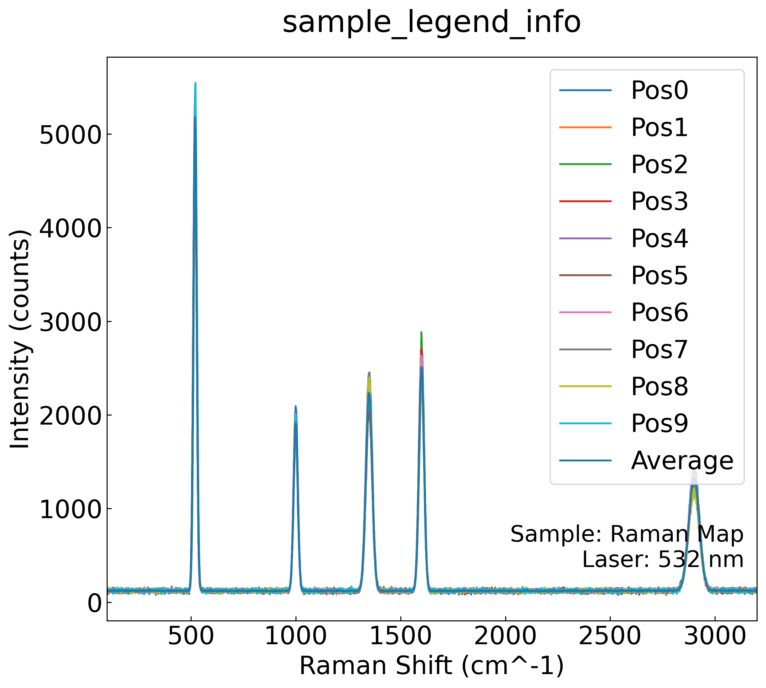
--legend-info で凡例付近にメタ情報を追記するラマン分光データの例です。

データの概要

ラマン分光のダミーデータを想定しています。横軸 Raman Shift (cm⁻¹) に対して、Pos0~Pos10 の各測定位置での Intensity (counts)(スペクトル強度)を並べています。

1
2
3
4
5
6
7
Raman Shift (cm^-1),Pos0: Intensity (counts),Pos1: Intensity (counts),Pos2: Intensity (counts),Pos3: Intensity (counts),Pos4: Intensity (counts),Pos5: Intensity (counts),Pos6: Intensity (counts),Pos7: Intensity (counts),Pos8: Intensity (counts),Pos9: Intensity (counts),Average: Intensity (counts)
100.0,117.0,124.0,134.0,135.0,111.0,126.0,132.0,116.0,126.0,114.0,124.0
101.551,117.0,126.0,106.0,138.0,110.0,127.0,134.0,146.0,134.0,116.0,125.0
103.102,126.0,139.0,110.0,150.0,119.0,134.0,128.0,128.0,116.0,141.0,129.0
104.652,100.0,108.0,90.0,119.0,118.0,145.0,106.0,117.0,144.0,117.0,116.0
106.203,102.0,87.0,114.0,125.0,117.0,108.0,112.0,117.0,133.0,136.0,115.0
...

Overlay: raman_max_legend_items

ディレクトリ構成

実行前のディレクトリ構成

1
2
3
sample8/
├── data.csv
└── sample_legend_info.py

実行例

 1
 2
 3
 4
 5
 6
 7
 8
 9
10
11
# sample_legend_info.py
from pathlib import Path
from rdetoolkit.graph import csv2graph

if __name__ == "__main__":
    csv2graph(
        csv_path=Path("sample8/data.csv"),
        title="sample_legend_info",
        legend_info="Sample: Raman Map\nLaser: 532 nm",
        no_individual=True,
    )
1
2
3
4
rdetoolkit csv2graph sample8/data.csv \
  --title "sample_legend_info" \
  --legend-info "Sample: Raman Map\nLaser: 532 nm" \
  --no-individual

オプションの説明

  • legend_info: 凡例枠の近く(もしくは右上)に任意テキストを追記します。複数行は \n で改行できます。
  • no_individual=True: オーバーレイ画像のみを生成し、個別プロットを省略します。

サンプル9: グリッド線の表示

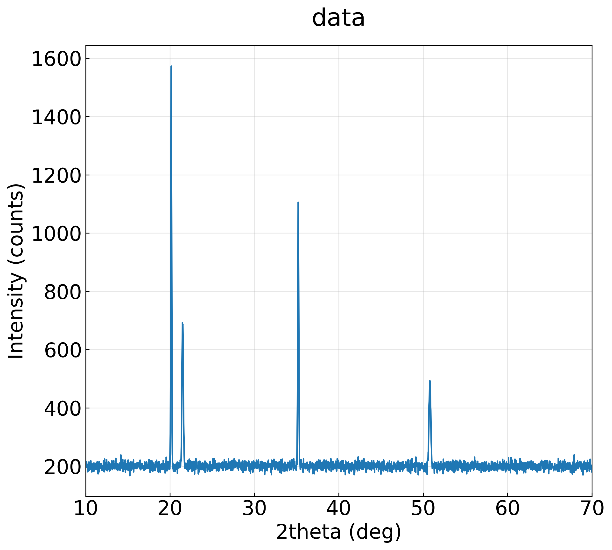
XRD データで --grid を有効にし、読み取りやすさを高めるサンプルです。

データの概要

サンプル:XRD 強度データを使って、グリッド線表示オプションを紹介します。

1
2
3
4
2theta (deg),Intensity (counts)
10.0,204.9671
10.02,198.6174
...

Overlay: raman_max_legend_items

ディレクトリ構成

実行前のディレクトリ構成

1
2
3
4
sample9/
├── cmd.md
├── data.csv
└── sample_grid.py

実行例

 1
 2
 3
 4
 5
 6
 7
 8
 9
10
# sample_grid.py
from pathlib import Path
from rdetoolkit.graph import csv2graph

if __name__ == "__main__":
    csv2graph(
        csv_path=Path("sample9/data.csv"),
        grid=True,                # --grid
        no_individual=True,
    )
1
2
3
rdetoolkit csv2graph sample9/data.csv \
  --grid \
  --no-individual

オプションの説明

  • grid=True, --grid : プロットに縦横のグリッド線を表示します。ピーク位置や値の読み取りがしやすくなります。
  • no_individual=True : 個別グラフを出力せず、オーバーレイ画像のみ生成します。

サンプル10: 表示範囲を絞り込む (xlim/ylim)

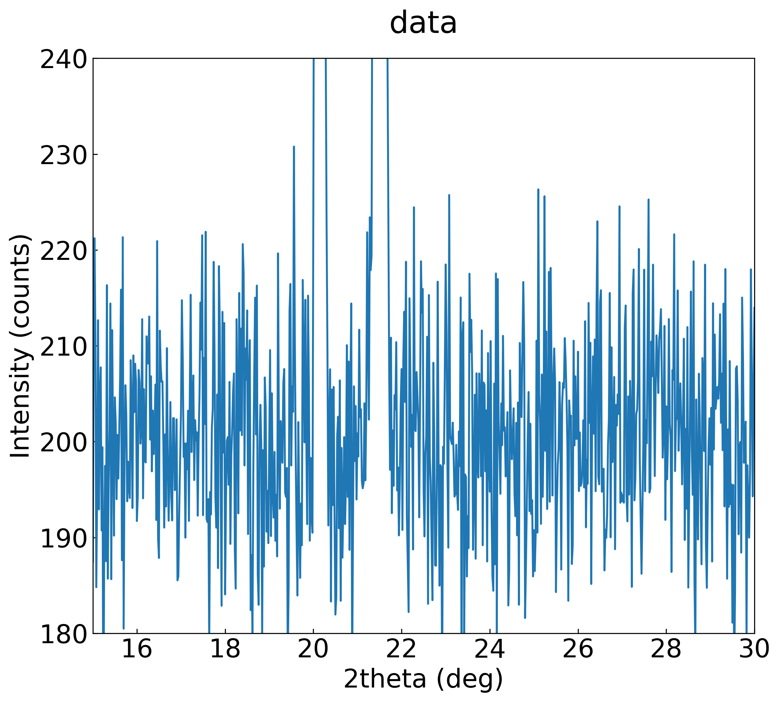
XRD データで --xlim--ylim を指定してピーク付近だけを拡大する例です。

データの概要

サンプル:XRD 強度データを使って、表示範囲を --xlim / --ylim で絞り込む方法を紹介します。

1
2
3
4
2theta (deg),Intensity (counts)
10.0,204.9671
10.02,198.6174
...

Overlay: raman_max_legend_items

ディレクトリ構成

実行前のディレクトリ構成

1
2
3
4
sample10/
├── cmd.md
├── data.csv
└── sample_lim.py

実行例

 1
 2
 3
 4
 5
 6
 7
 8
 9
10
11
# sample_lim.py
from pathlib import Path
from rdetoolkit.graph import csv2graph

if __name__ == "__main__":
    csv2graph(
        csv_path=Path("sample10/data.csv"),
        xlim=(15, 30),     # --xlim 15 30
        ylim=(180, 240),   # --ylim 180 240
        no_individual=True,
    )
1
2
3
4
rdetoolkit csv2graph sample10/data.csv \
  --xlim 15 30 \
  --ylim 180 240 \
  --no-individual

オプションの説明

  • --xlim <min> <max>, xlim=(<min>, <max>) : X 軸の表示範囲を指定します(単位は CSV の X 列と同じ)。例では 15°〜30° の 2θ のみを表示。
  • --ylim <min> <max>, ylim=(<min>, <max>) : Y 軸の表示範囲を指定します(単位は縦軸の列と同じ)。例では 180〜240 counts の強度のみを表示。
  • --no-individual : 個別グラフを生成せず、オーバーレイ画像のみ出力します。

表示範囲を絞ることで、ピーク付近の詳細を拡大表示したり、ノイズを除いた視認性を高めたりできます。

サンプル11: 代表画像と個別画像の出力先を分ける

--main-image-dir--output-dir を使って、代表画像と個別画像を別フォルダに保存する例です。

データの概要

サンプル:XRD 強度データを使って、代表画像と個別画像を別ディレクトリに保存する方法を紹介します。

1
2
3
4
2theta (deg),Intensity (counts)
10.0,204.9671
10.02,198.6174
...

Overlay: main

Overlay: other

ディレクトリ構成

1
2
3
4
$ ls -l sample11/
total 472
-rw-r--r--@ 1 user  staff  44132 10 26 23:33 data.csv
-rw-r--r--@ 1 user  staff    290 10 27 12:46 switch_output_directory.py

実行例

 1
 2
 3
 4
 5
 6
 7
 8
 9
10
# sample11/switch_output_directory.py
from pathlib import Path
from rdetoolkit.graph import csv2graph

if __name__ == "__main__":
    csv2graph(
        csv_path=Path("sample11/data.csv"),
        main_image_dir=Path("sample11/main_image"),   # --main-image-dir
        output_dir=Path("sample11/other_image"),      # --output-dir
    )
1
2
3
rdetoolkit csv2graph sample11/data.csv \
  --main-image-dir sample11/main_image \
  --output-dir sample11/other_image

実行結果と出力ファイル構成

1
2
3
4
5
6
7
sample11/
├── data.csv
├── main_image # 代表画像出力ディレクトリ   └── data.png
├── other_image # 個別画像出力ディレクトリ   └── data_intensity_(counts).png
└── switch_output_directory.py

オプションの説明

  • --main-image-dir : オーバーレイ画像を保存するディレクトリを指定します。デフォルトでは --output-dir と同じ場所になります。
  • --output-dir : 個別プロット(系列ごとの PNG)や HTML 出力を保存するディレクトリを指定します。指定がない場合は入力 CSV と同じフォルダに作成されます。

代表画像と個別画像を別フォルダに分けることで、レポート用の代表図と解析用の細かい図を整理しやすくなります。

サンプル12: Plotly HTML 出力を有効化

--html でインタラクティブな Plotly HTML を生成するサンプルです。

データの概要

サンプル:XRD 強度データを使って、Plotly によるインタラクティブ HTML を有効にする --html オプションを紹介します。

1
2
3
4
2theta (deg),Intensity (counts)
10.0,204.9671
10.02,198.6174
...

Overlay: png

ディレクトリ構成

1
2
3
sample12/
├── data.csv
└── output_html.py

実行例

 1
 2
 3
 4
 5
 6
 7
 8
 9
10
from pathlib import Path
from rdetoolkit.graph import csv2graph

if __name__ == "__main__":
    csv2graph(
        csv_path=Path("sample12/data.csv"),
        html=True,                 # --html
        output_dir=Path("plots"),
        no_individual=True,
    )
1
2
3
4
rdetoolkit csv2graph sample12/data.csv \
  --output-dir plots \
  --html \
  --no-individual

実行後ディレクトリ

1
2
3
4
5
6
sample12/
├── data.csv
├── data.html # 生成(HTMLはデフォルトでCSVと同じ場所)
├── output_html.py
└── plots/
    └── data.png # 生成

オプションの説明

  • --html : Plotly を使ったインタラクティブな HTML ファイル(*.html)を出力します。生成された HTML はブラウザで開き、マウス操作でズームやホバー表示が可能です。
  • --no-individual : 個別プロットをスキップし、統合プロットのみ生成します(HTML はデフォルトで CSV と同じ出力先に保存されます。必要に応じて --html-output-dir を指定してください)。

インタラクティブ出力を利用するには Plotly ライブラリがインストールされている必要があります。インストールされていないと、以下のようなエラーが出力されます。

1
2
3
ImportError: Plotly is required for HTML output but is not installed. Install it with: pip install plotly
🔥 Unexpected error: Plotly is required for HTML output but is not installed. Install it with: pip install plotly
Aborted!

サンプル14: 凡例配置ポリシー(legend_policy)の使い分け

12系列・3系列のダミーデータを使い、legend_policy の各値(legacy / auto / inside / outside_right / outside_bottom / hide)で凡例の配置がどう変わるかを比較するサンプルです。オプションの詳細は csvをグラフ化する の「凡例配置ポリシー」セクションを参照してください。

outside_right / outside_bottom では、プロット領域を縮小して凡例スペースを作るのではなく、凡例のサイズに応じてキャンバス側が拡張されます。系列数が多くてもグラフ本体の描画サイズは維持されます。

データの概要

12系列の data.csv と、3系列の data_few.csv を使用します。いずれも単調増加のダミー系列です。

1
2
3
4
x,series_01,series_02,series_03,series_04,series_05,series_06,series_07,series_08,series_09,series_10,series_11,series_12
0,0.0,0.4,1.0,1.5,1.9,2.4,3.0,3.5,4.0,4.5,5.0,5.5
1,0.6,1.2,1.6,2.1,2.6,3.1,3.6,4.1,4.6,5.1,5.7,6.1
...

準備: ダミーデータの生成

CSV は上記リンクからダウンロードできます。手元で生成する場合は、以下のスクリプトを実行してください(掲載データ・グラフはこのスクリプトで生成したものです)。

 1
 2
 3
 4
 5
 6
 7
 8
 9
10
11
12
13
14
15
16
17
18
19
20
21
22
23
24
25
26
27
28
29
30
31
32
33
34
35
36
37
38
# make_data.py
# Generate dummy CSV files for the legend_policy samples.
# data.csv: 12 increasing series / data_few.csv: 3 increasing series
from pathlib import Path

import numpy as np

BASE = Path(__file__).parent
RNG = np.random.default_rng(42)


def make_series_csv(path: Path, columns: list[str], offsets: list[float], slopes: list[float]) -> None:
    x = np.arange(11)
    header = ",".join(["x", *columns])
    lines = [header]
    for xi in x:
        values = [
            offset + slope * xi + RNG.normal(0, 0.05)
            for offset, slope in zip(offsets, slopes)
        ]
        lines.append(",".join([str(xi), *[f"{v:.1f}" for v in values]]))
    path.write_text("\n".join(lines) + "\n", encoding="utf-8")


if __name__ == "__main__":
    make_series_csv(
        BASE / "data.csv",
        columns=[f"series_{i:02d}" for i in range(1, 13)],
        offsets=[0.5 * i for i in range(12)],
        slopes=[0.6] * 12,
    )
    make_series_csv(
        BASE / "data_few.csv",
        columns=["series_alpha", "series_beta", "series_gamma"],
        offsets=[0.0, 1.0, 2.0],
        slopes=[0.8, 0.8, 0.8],
    )
    print("generated: data.csv, data_few.csv")
1
python sample14/make_data.py

ディレクトリ構成

1
2
3
4
5
sample14/
├── data.csv
├── data_few.csv
├── make_data.py
└── sample_legend_policy.py

同梱の sample_legend_policy.py を実行すると、以下の全ケースの PNG をまとめて生成できます。以降は各ケースを個別に実行する例です。

ケース1: legacy(従来動作)

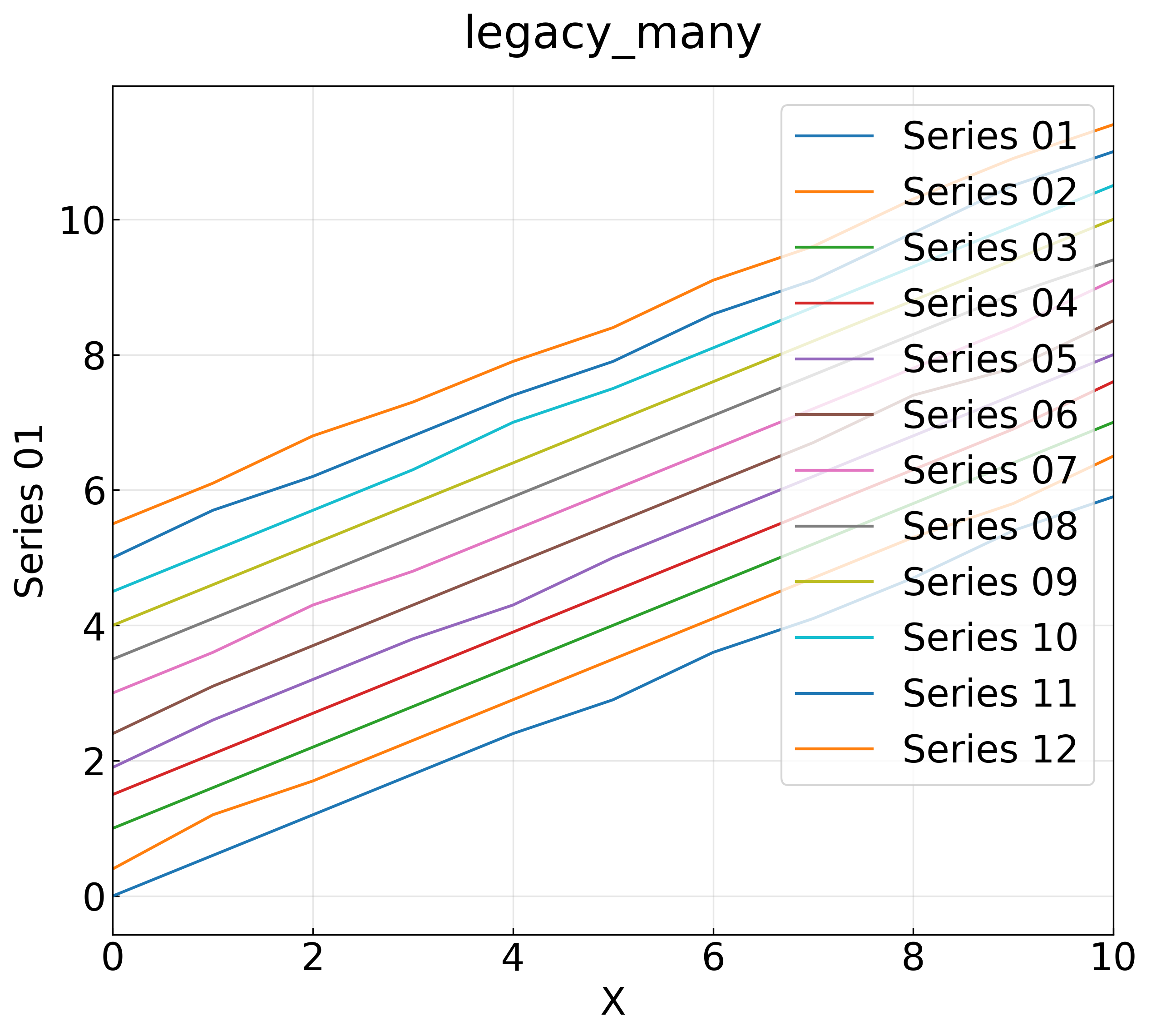
legend_policy を指定しない場合のデフォルトです。legend_locmax_legend_items による従来の凡例制御が維持され、凡例はプロット領域内に描画されます。
legacy_many

 1
 2
 3
 4
 5
 6
 7
 8
 9
10
11
12
13
14
15
from pathlib import Path
from rdetoolkit.graph import csv2graph

if __name__ == "__main__":
    csv2graph(
        csv_path=Path("sample14/data.csv"),
        output_dir=Path("sample14"),
        x_col="x",
        no_individual=True,
        grid=True,
        title="legacy_many",
        legend_policy="legacy",
        legend_loc="upper right",
        max_legend_items=30,
    )
1
2
3
4
5
6
7
8
rdetoolkit csv2graph sample14/data.csv \
  --output-dir sample14 \
  --x-col x \
  --no-individual --grid \
  --title legacy_many \
  --legend-policy legacy \
  --legend-loc "upper right" \
  --max-legend-items 30

ケース2: auto × 3系列(プロット内に表示)

auto は凡例項目数で配置を自動選択します。3系列は legend_outside_threshold(デフォルト8)以下なので、凡例はプロット領域内(inside)に置かれます。
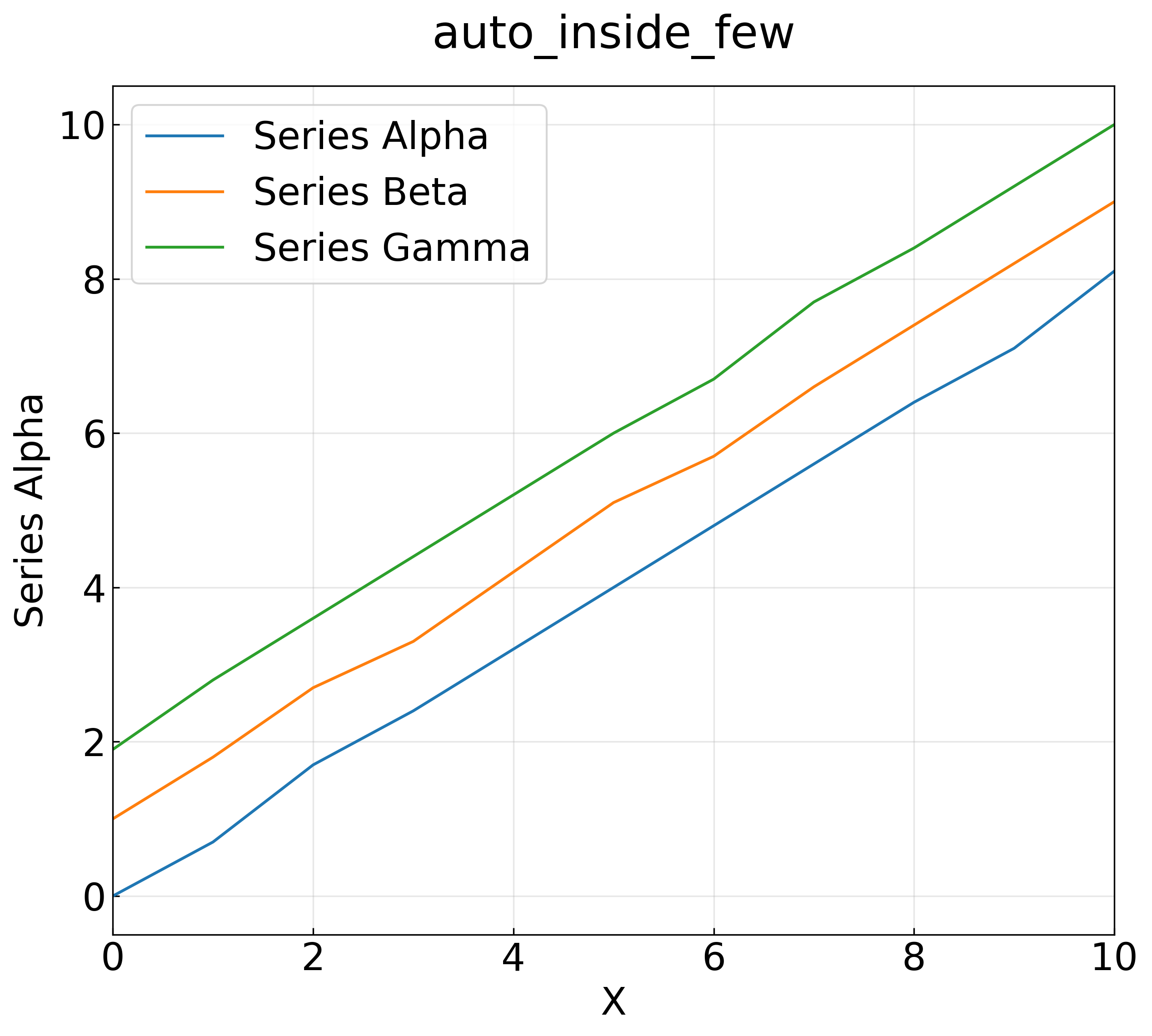
auto_inside_few

 1
 2
 3
 4
 5
 6
 7
 8
 9
10
11
12
13
14
15
from pathlib import Path
from rdetoolkit.graph import csv2graph

if __name__ == "__main__":
    csv2graph(
        csv_path=Path("sample14/data_few.csv"),
        output_dir=Path("sample14"),
        x_col="x",
        no_individual=True,
        grid=True,
        title="auto_inside_few",
        legend_policy="auto",
        legend_outside_threshold=8,
        max_legend_items=20,
    )
1
2
3
4
5
6
7
8
rdetoolkit csv2graph sample14/data_few.csv \
  --output-dir sample14 \
  --x-col x \
  --no-individual --grid \
  --title auto_inside_few \
  --legend-policy auto \
  --legend-outside-threshold 8 \
  --max-legend-items 20

ケース3: auto × 12系列(右外側に自動切り替え)

12系列は legend_outside_threshold=8 を超えるため、auto が凡例を右外側(outside_right)へ自動的に移動します。プロット領域のサイズは維持され、キャンバスが右へ拡張されます。
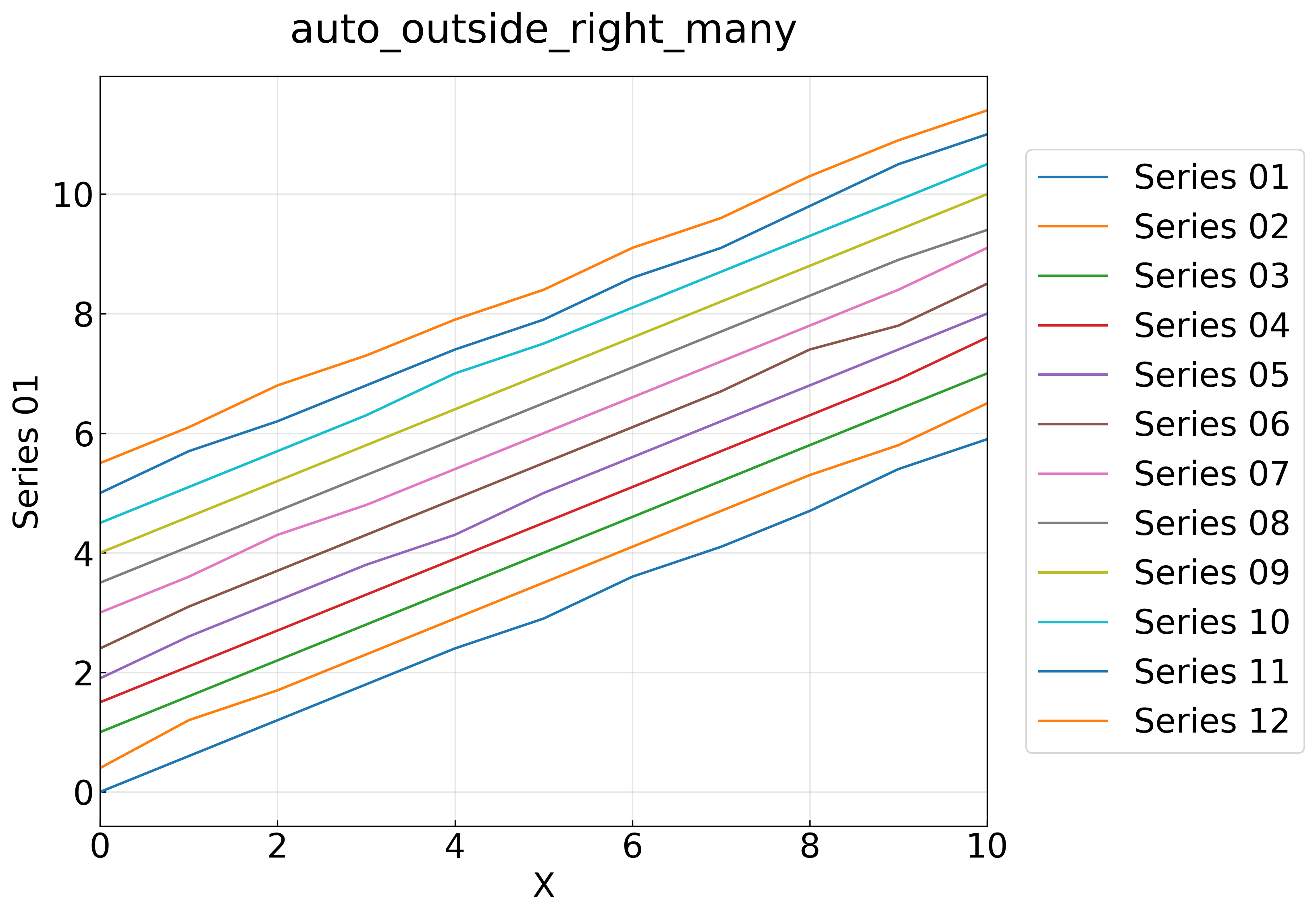
auto_outside_right_many

 1
 2
 3
 4
 5
 6
 7
 8
 9
10
11
12
13
14
15
from pathlib import Path
from rdetoolkit.graph import csv2graph

if __name__ == "__main__":
    csv2graph(
        csv_path=Path("sample14/data.csv"),
        output_dir=Path("sample14"),
        x_col="x",
        no_individual=True,
        grid=True,
        title="auto_outside_right_many",
        legend_policy="auto",
        legend_outside_threshold=8,
        max_legend_items=30,
    )
1
2
3
4
5
6
7
8
rdetoolkit csv2graph sample14/data.csv \
  --output-dir sample14 \
  --x-col x \
  --no-individual --grid \
  --title auto_outside_right_many \
  --legend-policy auto \
  --legend-outside-threshold 8 \
  --max-legend-items 30

ケース4: outside_right を強制

項目数に関係なく、凡例を常にプロット右外側へ配置します。
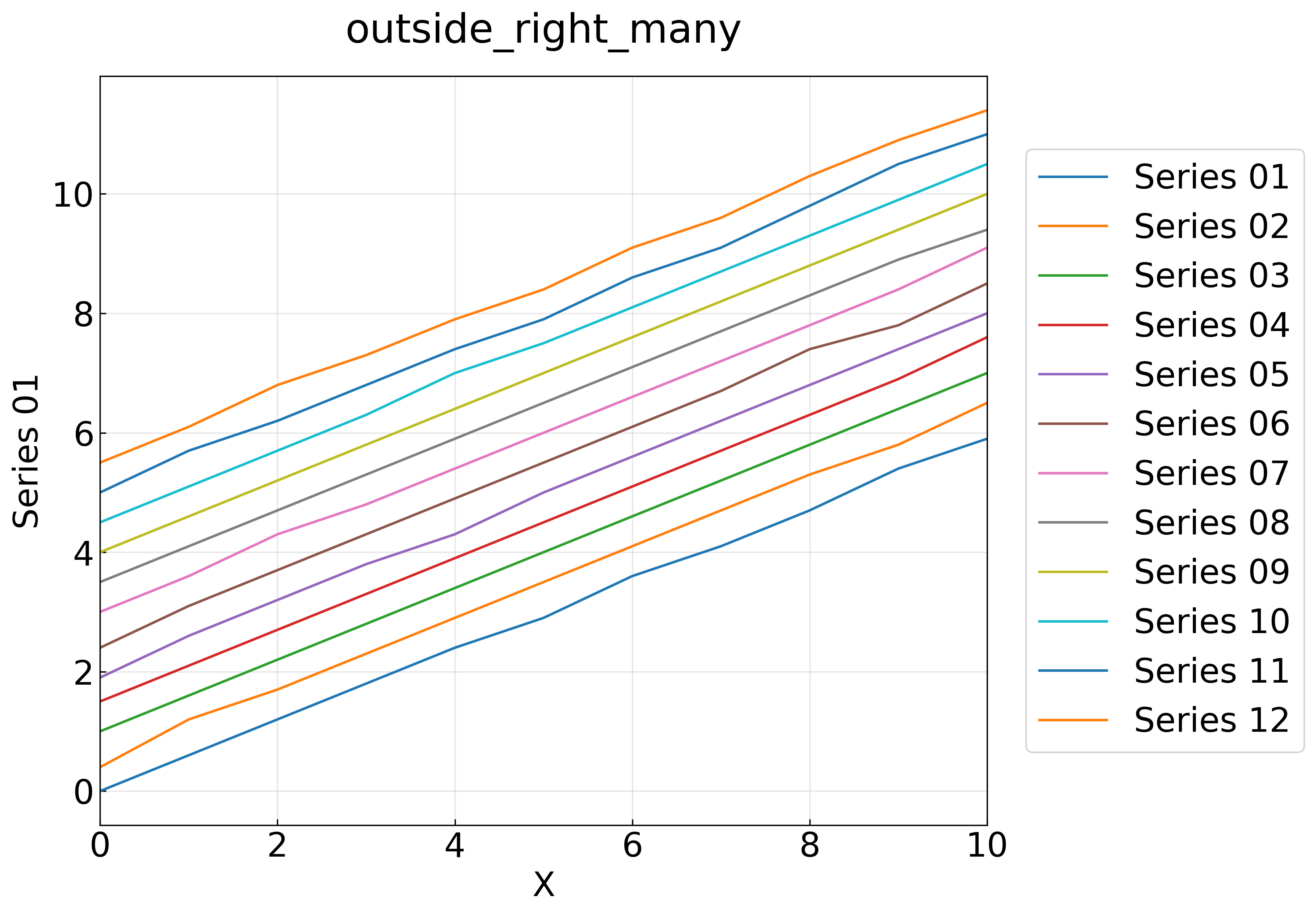
outside_right_many

 1
 2
 3
 4
 5
 6
 7
 8
 9
10
11
12
13
14
from pathlib import Path
from rdetoolkit.graph import csv2graph

if __name__ == "__main__":
    csv2graph(
        csv_path=Path("sample14/data.csv"),
        output_dir=Path("sample14"),
        x_col="x",
        no_individual=True,
        grid=True,
        title="outside_right_many",
        legend_policy="outside_right",
        max_legend_items=30,
    )
1
2
3
4
5
6
7
rdetoolkit csv2graph sample14/data.csv \
  --output-dir sample14 \
  --x-col x \
  --no-individual --grid \
  --title outside_right_many \
  --legend-policy outside_right \
  --max-legend-items 30

ケース5: outside_bottom + legend_ncol=4

凡例をグラフ下側に4列で配置します。段数は 列数 = legend_ncol から自動的に決まります(12項目 ÷ 4列 = 3段)。
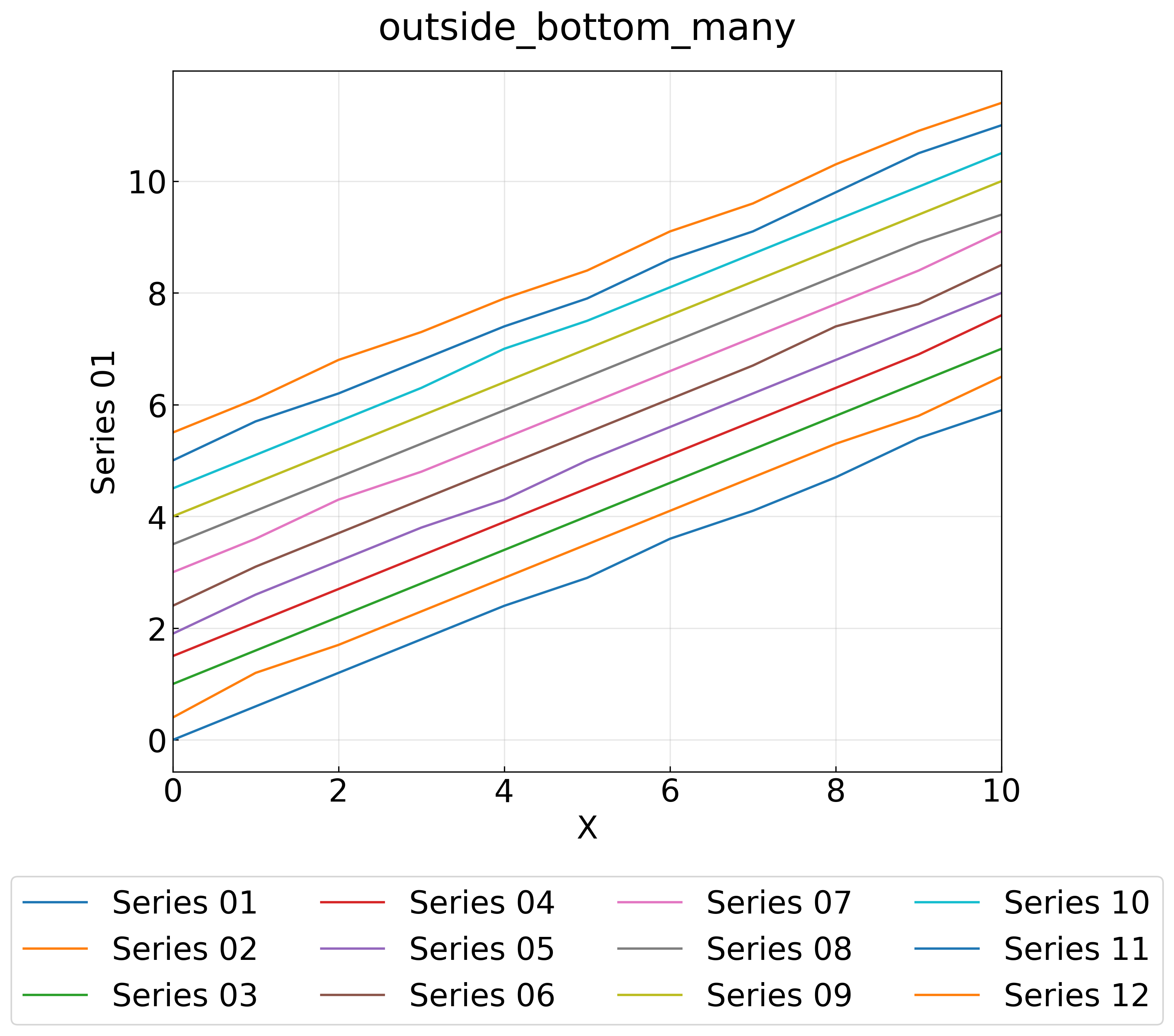
outside_bottom_many

 1
 2
 3
 4
 5
 6
 7
 8
 9
10
11
12
13
14
15
from pathlib import Path
from rdetoolkit.graph import csv2graph

if __name__ == "__main__":
    csv2graph(
        csv_path=Path("sample14/data.csv"),
        output_dir=Path("sample14"),
        x_col="x",
        no_individual=True,
        grid=True,
        title="outside_bottom_many",
        legend_policy="outside_bottom",
        legend_ncol=4,
        max_legend_items=30,
    )
1
2
3
4
5
6
7
8
rdetoolkit csv2graph sample14/data.csv \
  --output-dir sample14 \
  --x-col x \
  --no-individual --grid \
  --title outside_bottom_many \
  --legend-policy outside_bottom \
  --legend-ncol 4 \
  --max-legend-items 30

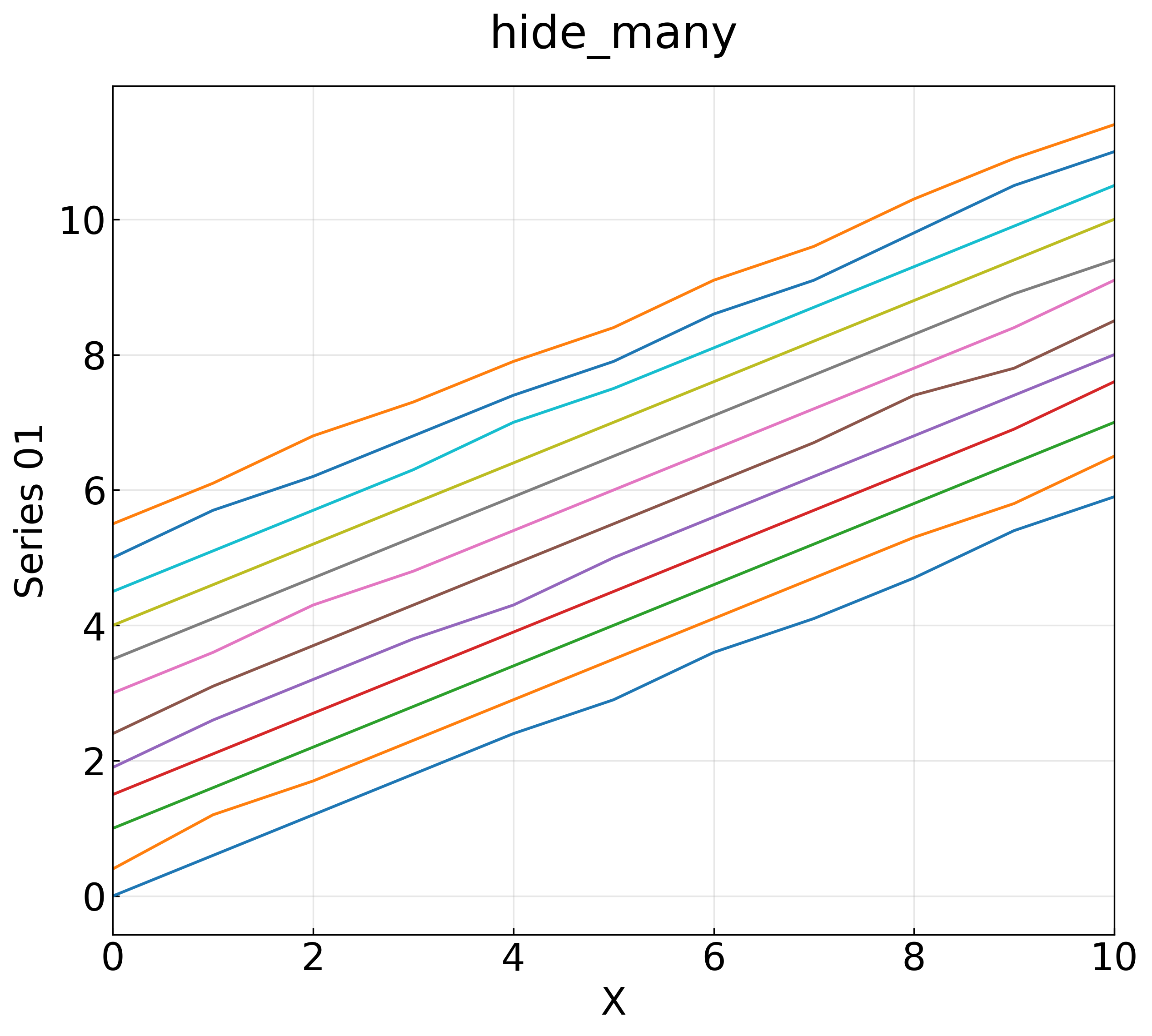
ケース6: hide(凡例を表示しない)

hide_many

 1
 2
 3
 4
 5
 6
 7
 8
 9
10
11
12
13
14
from pathlib import Path
from rdetoolkit.graph import csv2graph

if __name__ == "__main__":
    csv2graph(
        csv_path=Path("sample14/data.csv"),
        output_dir=Path("sample14"),
        x_col="x",
        no_individual=True,
        grid=True,
        title="hide_many",
        legend_policy="hide",
        max_legend_items=30,
    )
1
2
3
4
5
6
7
rdetoolkit csv2graph sample14/data.csv \
  --output-dir sample14 \
  --x-col x \
  --no-individual --grid \
  --title hide_many \
  --legend-policy hide \
  --max-legend-items 30

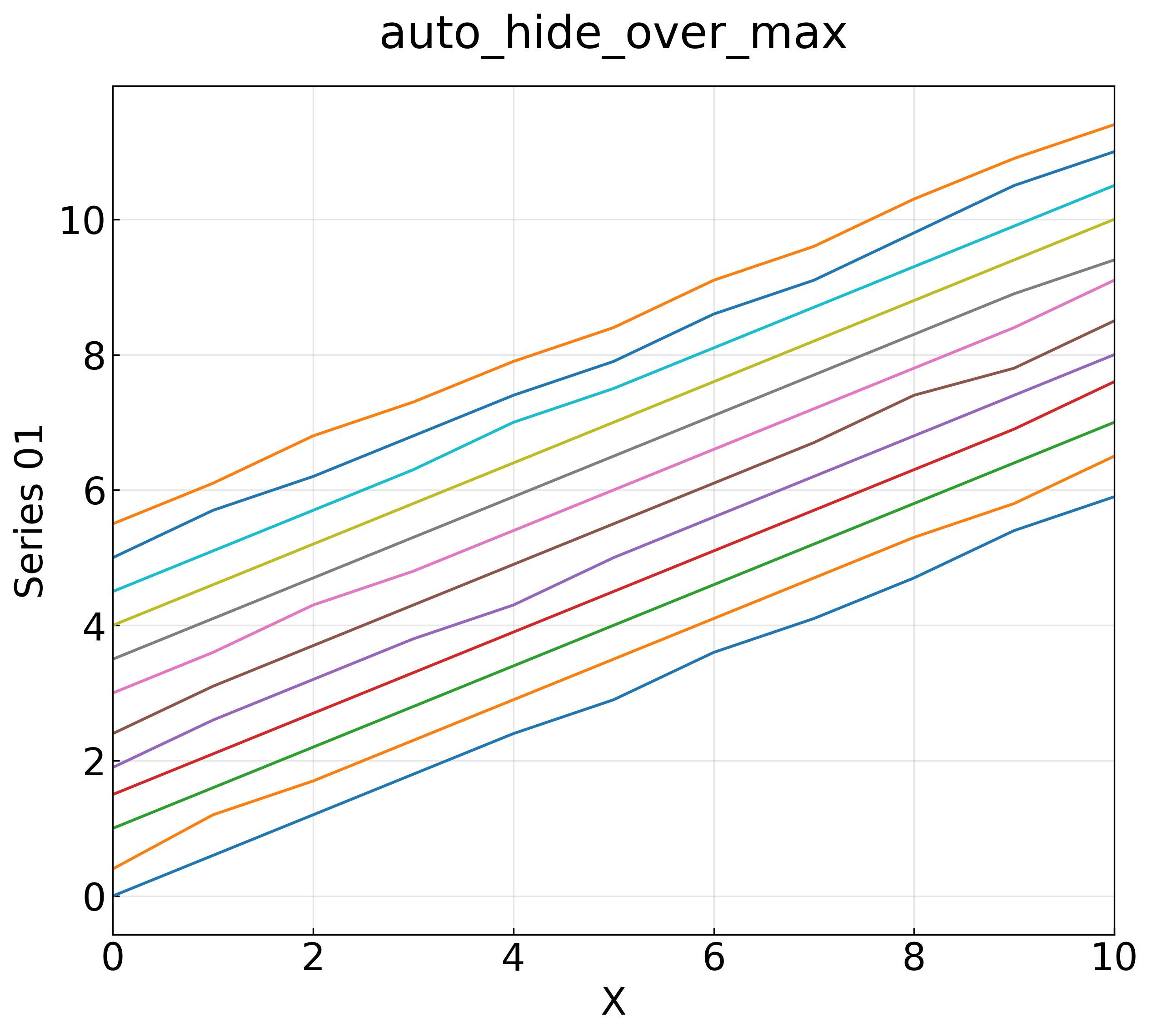
ケース7: auto × max_legend_items 超過(自動非表示)

12系列に対して max_legend_items=5 を指定すると、上限超過により auto が凡例を非表示にします。
auto_hide_over_max

 1
 2
 3
 4
 5
 6
 7
 8
 9
10
11
12
13
14
15
from pathlib import Path
from rdetoolkit.graph import csv2graph

if __name__ == "__main__":
    csv2graph(
        csv_path=Path("sample14/data.csv"),
        output_dir=Path("sample14"),
        x_col="x",
        no_individual=True,
        grid=True,
        title="auto_hide_over_max",
        legend_policy="auto",
        legend_outside_threshold=8,
        max_legend_items=5,
    )
1
2
3
4
5
6
7
8
rdetoolkit csv2graph sample14/data.csv \
  --output-dir sample14 \
  --x-col x \
  --no-individual --grid \
  --title auto_hide_over_max \
  --legend-policy auto \
  --legend-outside-threshold 8 \
  --max-legend-items 5

オプションの説明

  • legend_policy, --legend-policy : 凡例の配置ポリシー。legacy(デフォルト・従来動作)/ auto(項目数で自動選択)/ inside / outside_right / outside_bottom / hide から選択します。
  • legend_outside_threshold, --legend-outside-threshold : auto がプロット内から右外側配置へ切り替える項目数のしきい値(デフォルト8。この値を超えると切り替え)。
  • legend_ncol, --legend-ncol : outside_bottom の凡例列数(未指定時は3列)。
  • max_legend_items, --max-legend-items : 凡例の最大表示項目数。超過すると凡例が非表示になります(auto 以外の明示ポリシーでも適用)。
  • x_col="x", --x-col x : X 軸列を列名で指定。y_cols を省略すると残りの全列が Y 系列になります。

サンプル15: 30系列以上の高密度凡例と自動配置

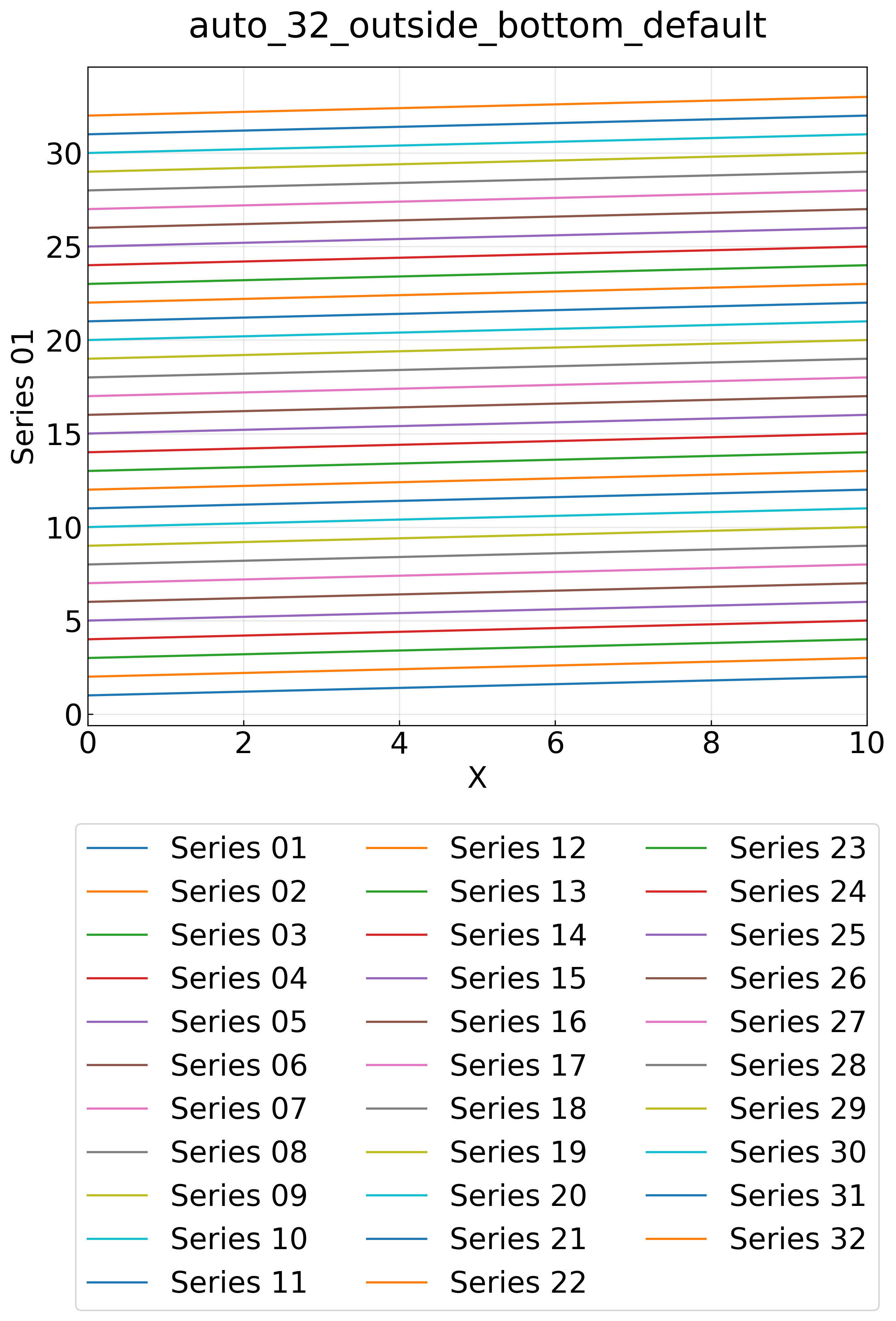
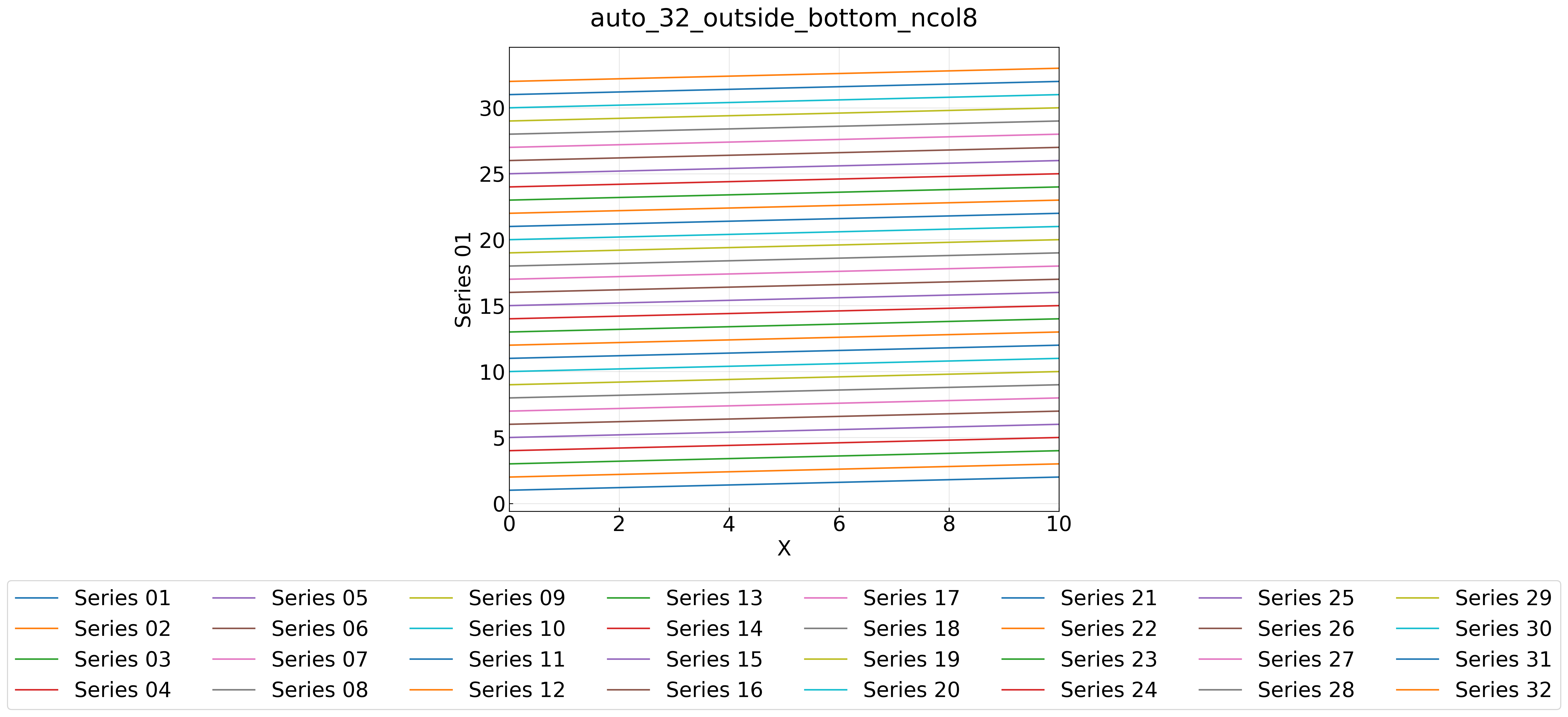
32系列のダミーデータを使い、凡例項目が非常に多い場合の配置制御を確認するサンプルです。legend_bottom_threshold(デフォルト21)により、21項目以上では auto が凡例をグラフ下側へ自動配置します。

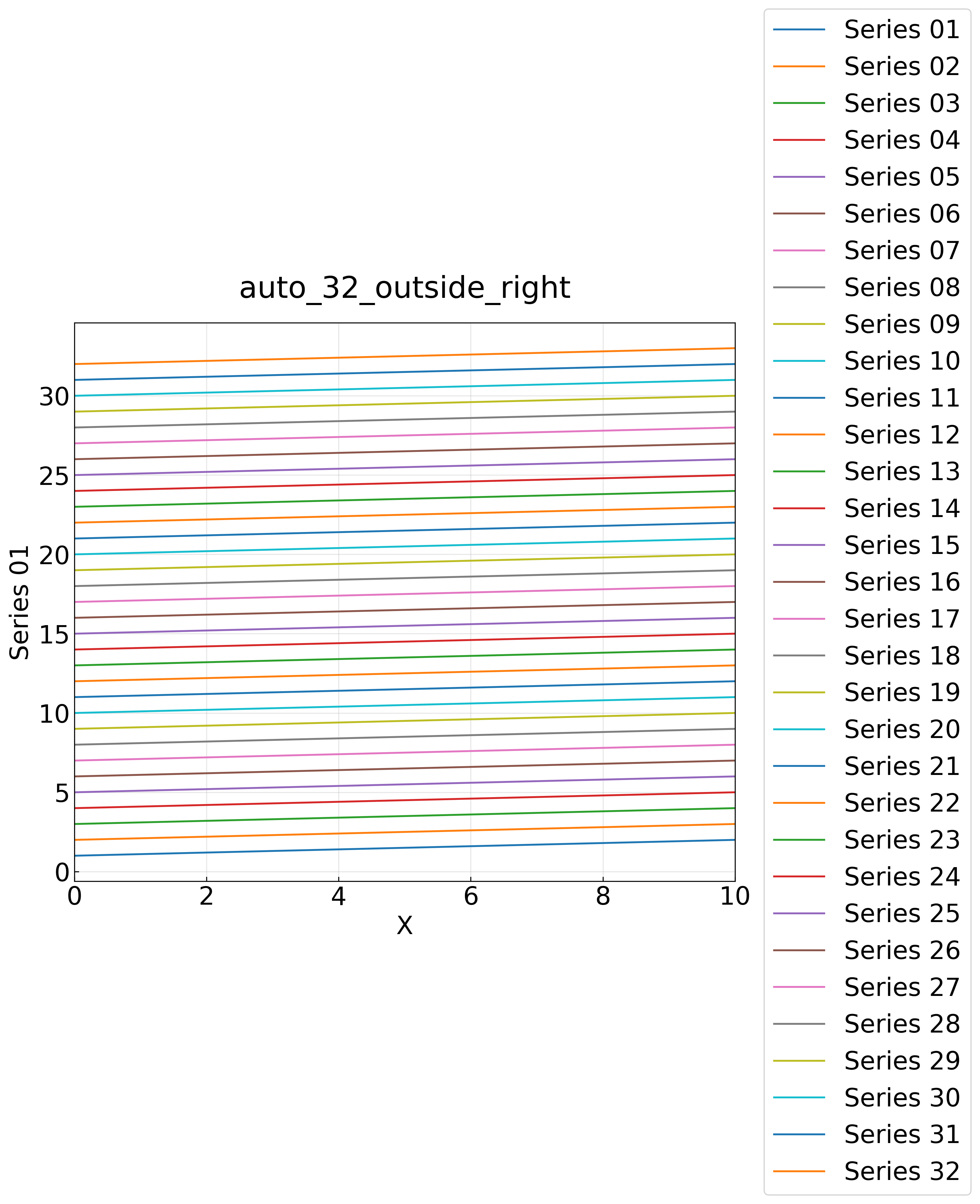
いずれのケースでもグラフ本体(プロット領域)のサイズは維持され、凡例のサイズに応じてキャンバス側が拡張されます。保存された PNG/SVG で凡例が見切れることはありません。

データの概要

32系列の直線データです。各系列は series_i(x) = i + 0.1 × x(x = 0〜10)で完全に再現できます。

1
2
3
4
x,series_01,series_02,...,series_32
0,1.0,2.0,3.0,...,32.0
1,1.1,2.1,3.1,...,32.1
...

準備: ダミーデータの生成

以下のスクリプトで掲載データと同一の CSV を生成できます。

 1
 2
 3
 4
 5
 6
 7
 8
 9
10
11
12
13
14
15
# make_data.py
# Generate a dummy CSV with 32 series for dense-legend samples.
# Each series is a straight line: series_i(x) = i + 0.1 * x  (x = 0..10)
from pathlib import Path

BASE = Path(__file__).parent

if __name__ == "__main__":
    columns = [f"series_{i:02d}" for i in range(1, 33)]
    lines = [",".join(["x", *columns])]
    for x in range(11):
        values = [i + 0.1 * x for i in range(1, 33)]
        lines.append(",".join([str(x), *[f"{v:.1f}" for v in values]]))
    (BASE / "data.csv").write_text("\n".join(lines) + "\n", encoding="utf-8")
    print("generated: data.csv")
1
python sample15/make_data.py

ディレクトリ構成

1
2
3
4
sample15/
├── data.csv
├── make_data.py
└── sample_dense_legend.py

同梱の sample_dense_legend.py を実行すると、以下の全ケースの PNG をまとめて生成できます。

ケース1: auto のデフォルト動作(21項目以上 → 下側配置)

32系列はデフォルトの legend_bottom_threshold=21 以上なので、auto が凡例をグラフ下側へ配置します。列数はデフォルト3列、legend_ncol=8 を指定すると4段に圧縮できます。
auto_32_outside_bottom_default

auto_32_outside_bottom_ncol8

 1
 2
 3
 4
 5
 6
 7
 8
 9
10
11
12
13
14
15
16
from pathlib import Path
from rdetoolkit.graph import csv2graph

if __name__ == "__main__":
    csv2graph(
        csv_path=Path("sample15/data.csv"),
        output_dir=Path("sample15"),
        x_col="x",
        no_individual=True,
        grid=True,
        title="auto_32_outside_bottom_default",
        legend_policy="auto",
        legend_outside_threshold=8,
        max_legend_items=40,
        # legend_ncol=8,  # 8列(4段)にする場合
    )
1
2
3
4
5
6
7
8
9
rdetoolkit csv2graph sample15/data.csv \
  --output-dir sample15 \
  --x-col x \
  --no-individual --grid \
  --title auto_32_outside_bottom_default \
  --legend-policy auto \
  --legend-outside-threshold 8 \
  --max-legend-items 40
  # --legend-ncol 8  # 8列(4段)にする場合

ケース2: 下側切り替えを無効化して右外側に置く

legend_bottom_threshold=None(CLI では --legend-bottom-threshold 0)を指定すると下側への自動切り替えが無効になり、従来どおり右外側(outside_right)に配置されます。32項目の縦長凡例でも、キャンバスが上下にも拡張されるため見切れません。
auto_32_outside_right

 1
 2
 3
 4
 5
 6
 7
 8
 9
10
11
12
13
14
15
16
from pathlib import Path
from rdetoolkit.graph import csv2graph

if __name__ == "__main__":
    csv2graph(
        csv_path=Path("sample15/data.csv"),
        output_dir=Path("sample15"),
        x_col="x",
        no_individual=True,
        grid=True,
        title="auto_32_outside_right",
        legend_policy="auto",
        legend_outside_threshold=8,
        legend_bottom_threshold=None,
        max_legend_items=40,
    )
1
2
3
4
5
6
7
8
9
rdetoolkit csv2graph sample15/data.csv \
  --output-dir sample15 \
  --x-col x \
  --no-individual --grid \
  --title auto_32_outside_right \
  --legend-policy auto \
  --legend-outside-threshold 8 \
  --legend-bottom-threshold 0 \
  --max-legend-items 40

ケース3: legend_outside_threshold の境界動作

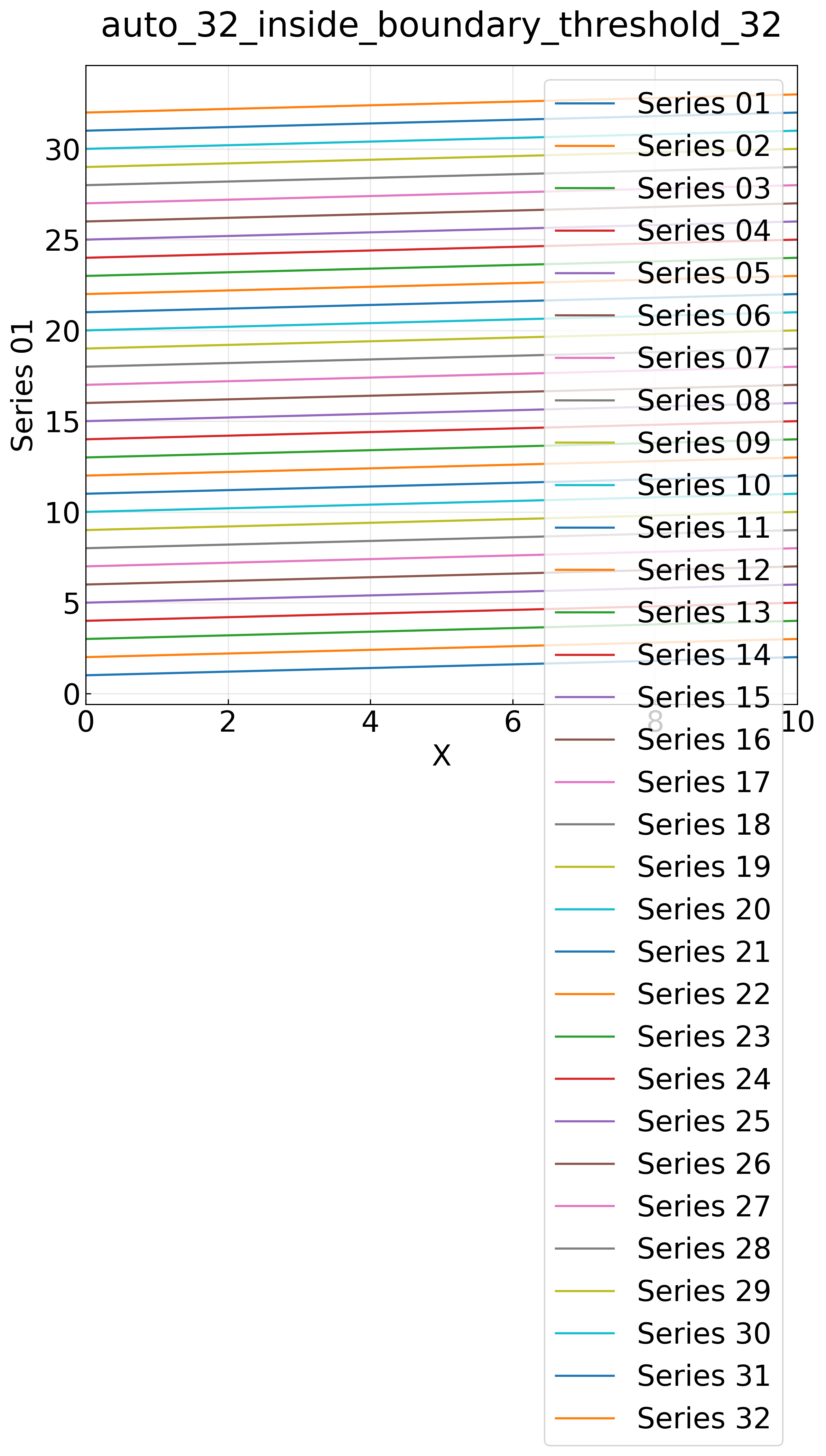
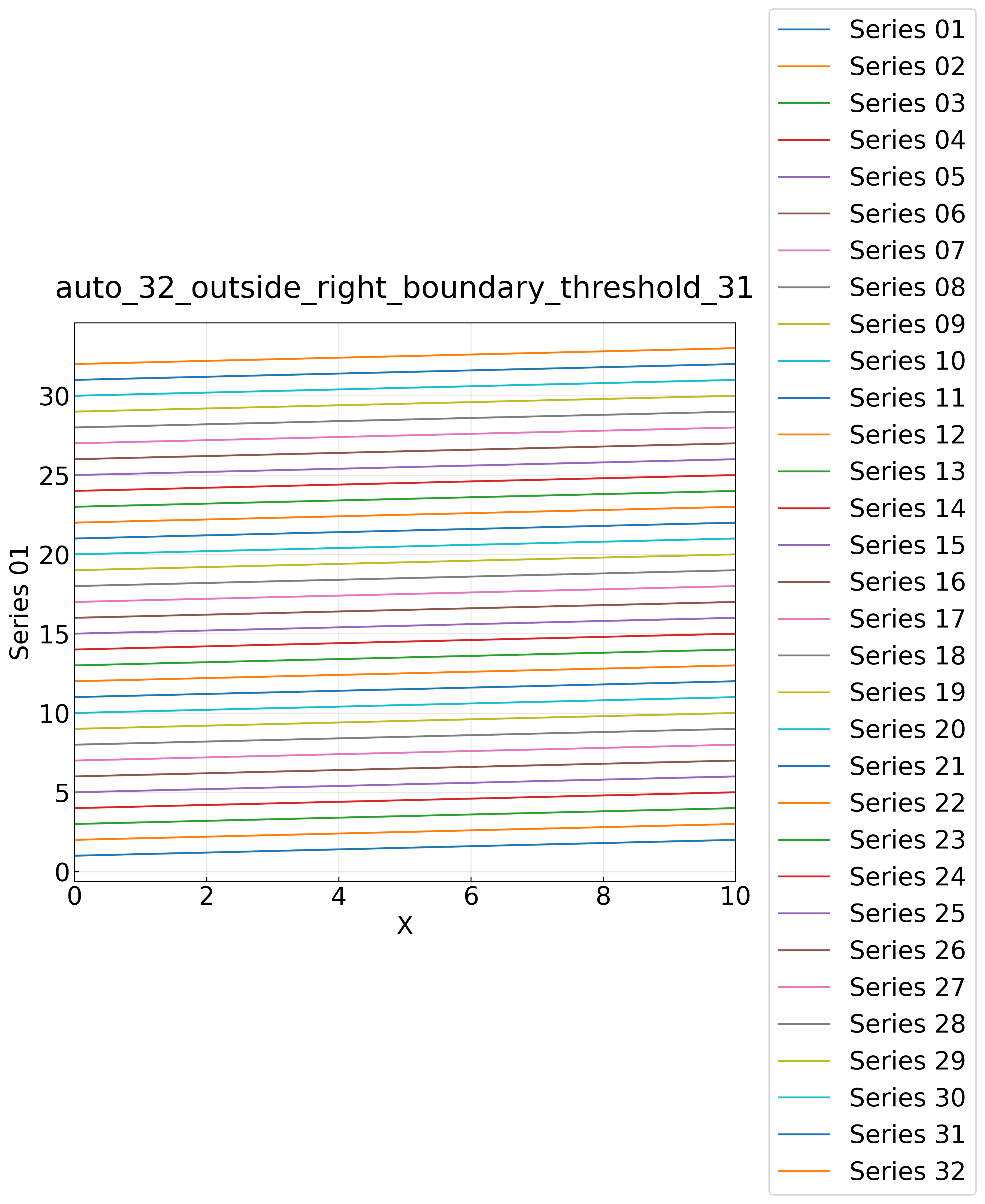
右外側への切り替えは「しきい値を超えたら」です。32系列に対してしきい値32なら inside のまま、31なら右外側へ切り替わります(下側切り替えは無効化して確認)。

しきい値32(inside のまま)のグラフは、32項目がプロット内に収まらず溢れる様子を示しています。多系列で inside 相当の配置を使うべきでない実例として掲載しています。

auto_32_inside_boundary_threshold_32

auto_32_outside_right_boundary_threshold_31

 1
 2
 3
 4
 5
 6
 7
 8
 9
10
11
12
13
14
15
16
17
from pathlib import Path
from rdetoolkit.graph import csv2graph

if __name__ == "__main__":
    for threshold in (32, 31):
        csv2graph(
            csv_path=Path("sample15/data.csv"),
            output_dir=Path("sample15"),
            x_col="x",
            no_individual=True,
            grid=True,
            title=f"auto_32_boundary_threshold_{threshold}",
            legend_policy="auto",
            legend_outside_threshold=threshold,
            legend_bottom_threshold=None,
            max_legend_items=40,
        )
1
2
3
4
5
6
7
8
9
rdetoolkit csv2graph sample15/data.csv \
  --output-dir sample15 \
  --x-col x \
  --no-individual --grid \
  --title auto_32_boundary_threshold_32 \
  --legend-policy auto \
  --legend-outside-threshold 32 \
  --legend-bottom-threshold 0 \
  --max-legend-items 40

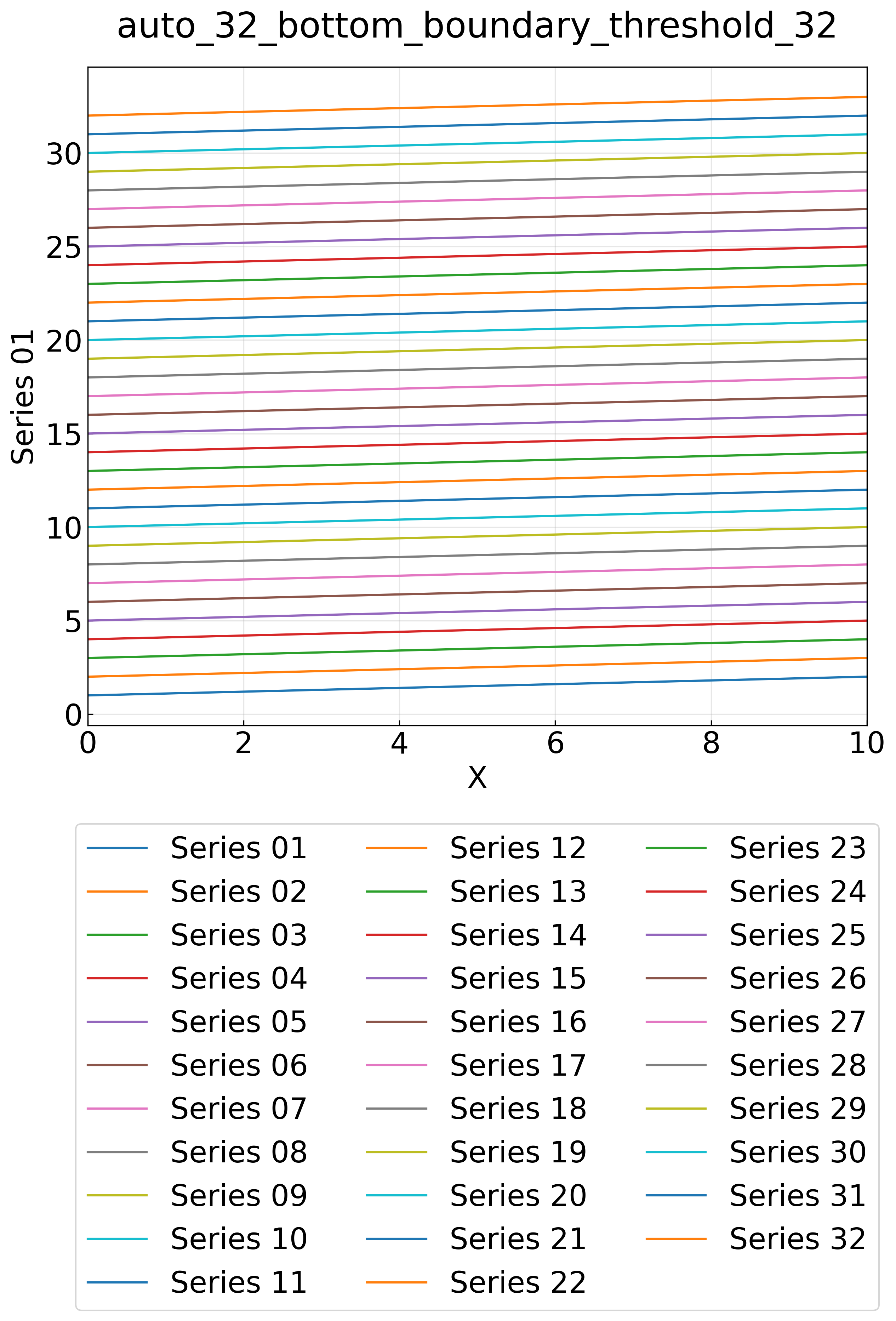
ケース4: legend_bottom_threshold の境界動作

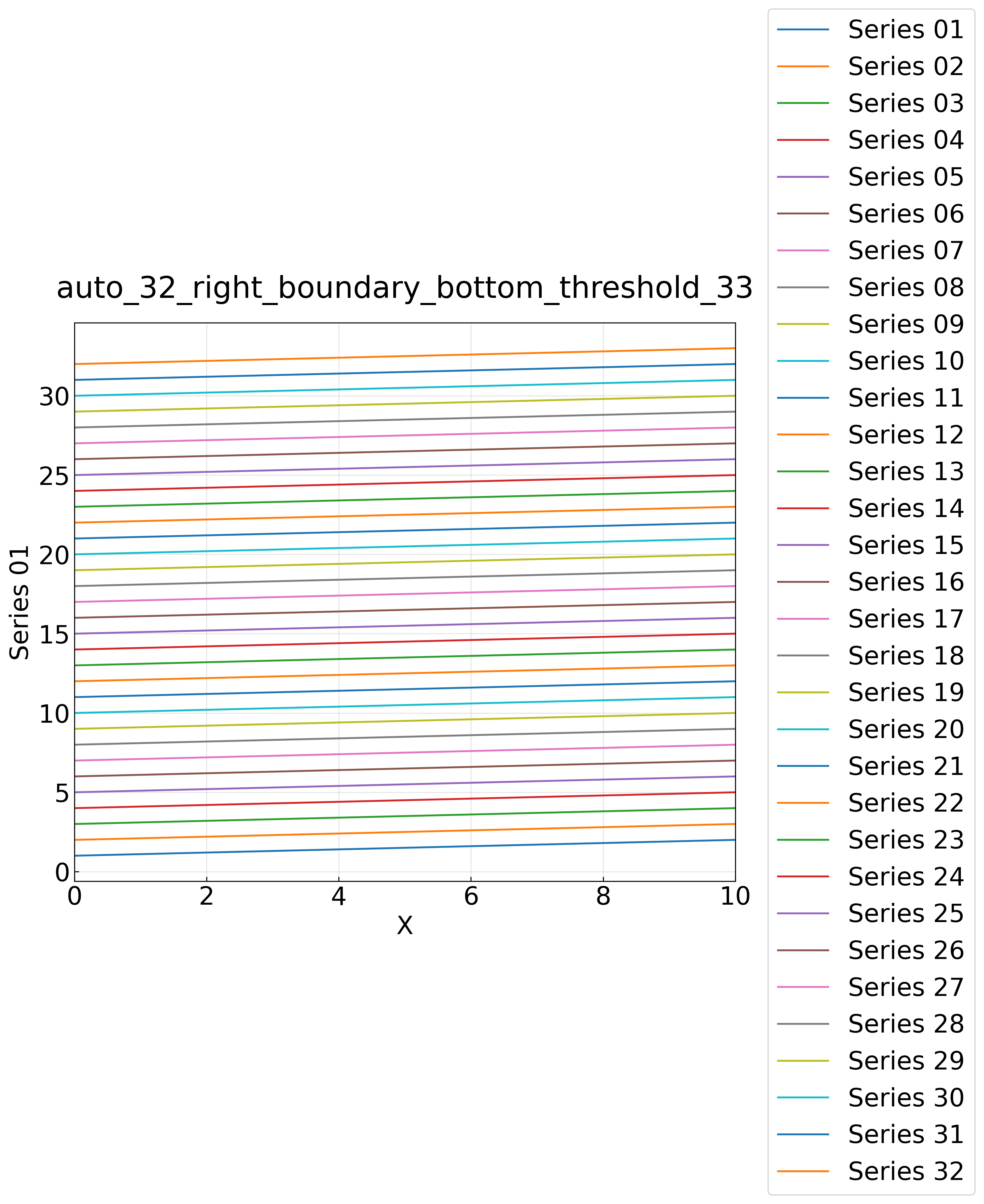
下側への切り替えは「しきい値以上」です。32系列に対してしきい値32なら下側へ、33なら右外側になります。
auto_32_bottom_boundary_threshold_32

auto_32_right_boundary_bottom_threshold_33

 1
 2
 3
 4
 5
 6
 7
 8
 9
10
11
12
13
14
15
16
17
from pathlib import Path
from rdetoolkit.graph import csv2graph

if __name__ == "__main__":
    for bottom_threshold in (32, 33):
        csv2graph(
            csv_path=Path("sample15/data.csv"),
            output_dir=Path("sample15"),
            x_col="x",
            no_individual=True,
            grid=True,
            title=f"auto_32_bottom_boundary_{bottom_threshold}",
            legend_policy="auto",
            legend_outside_threshold=8,
            legend_bottom_threshold=bottom_threshold,
            max_legend_items=40,
        )
1
2
3
4
5
6
7
8
9
rdetoolkit csv2graph sample15/data.csv \
  --output-dir sample15 \
  --x-col x \
  --no-individual --grid \
  --title auto_32_bottom_boundary_32 \
  --legend-policy auto \
  --legend-outside-threshold 8 \
  --legend-bottom-threshold 32 \
  --max-legend-items 40

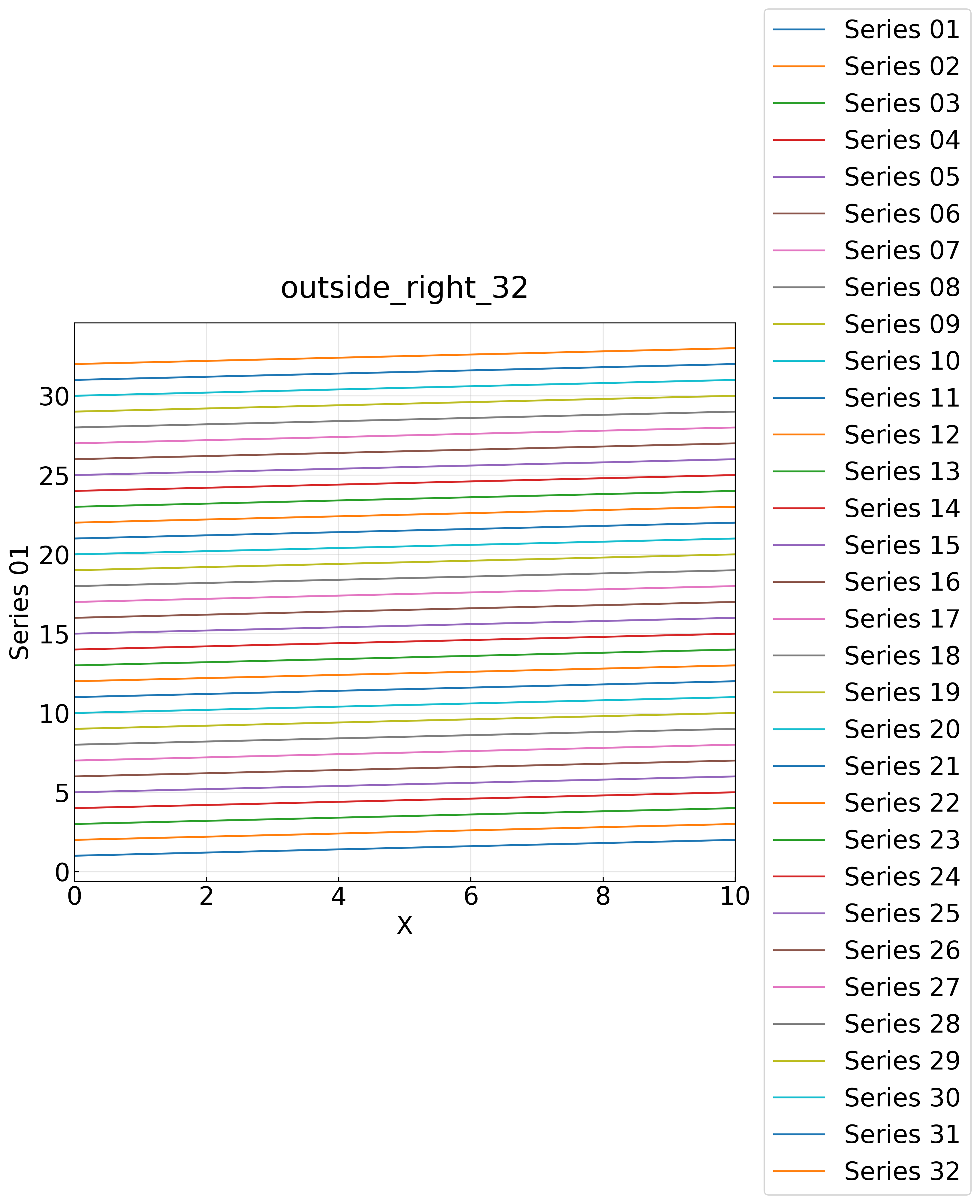
ケース5: 配置を強制する(outside_right / outside_bottom)

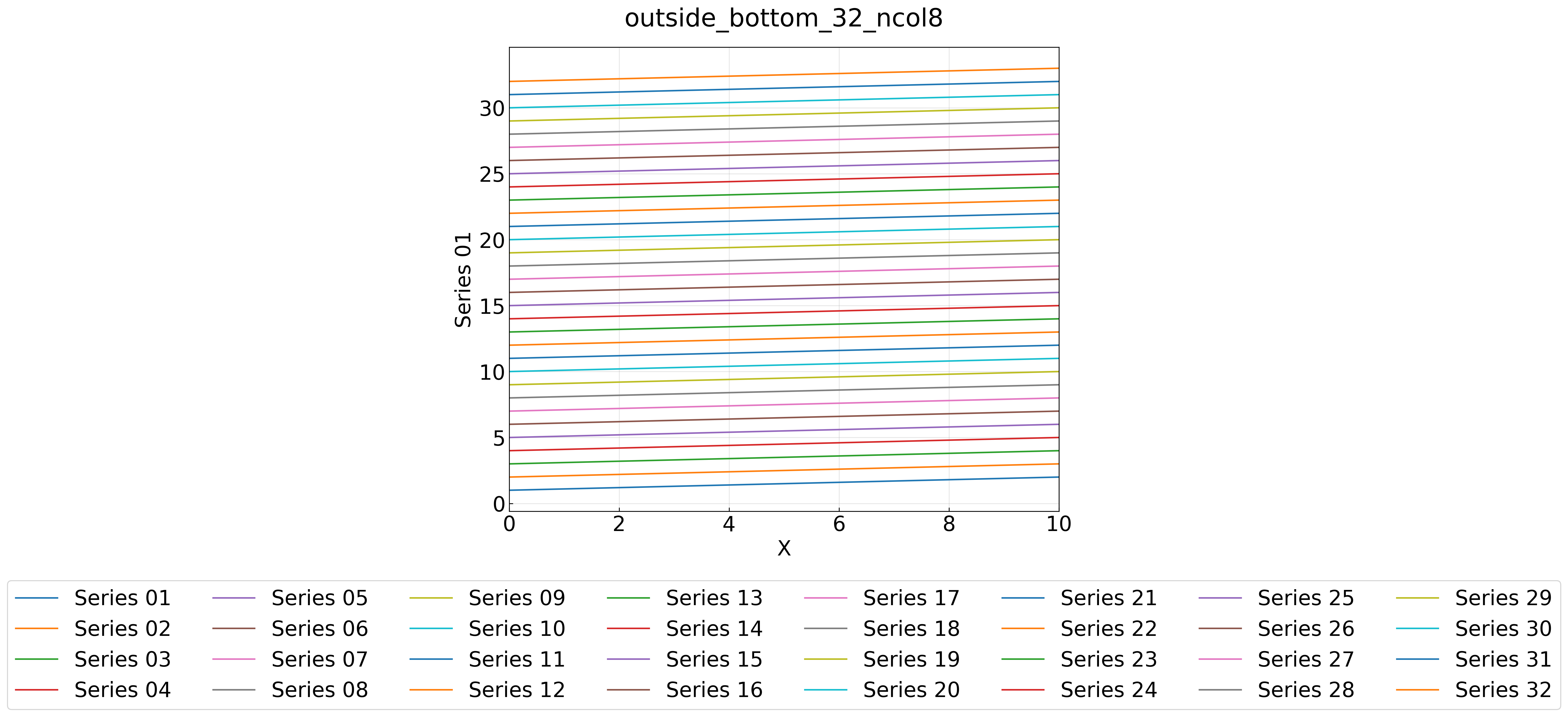
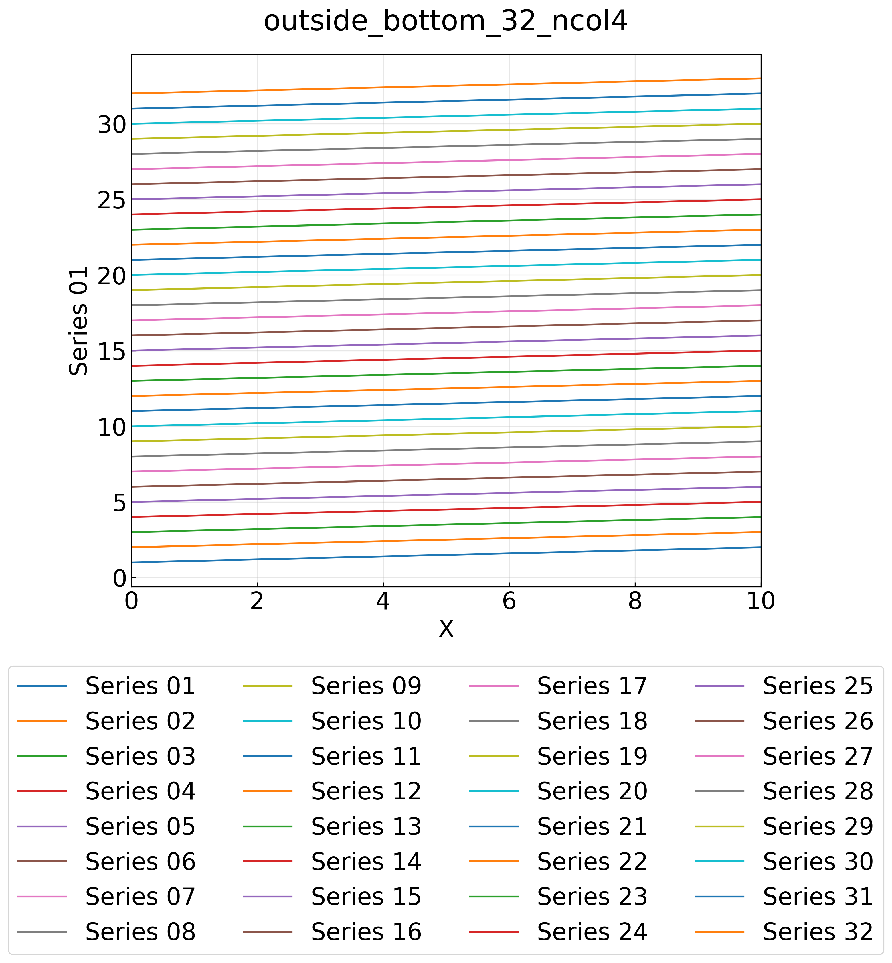
auto を使わず配置を明示指定する例です。outside_bottomlegend_ncol で列数(=段数)を制御できます。

outside_right_32

outside_bottom_32_ncol8

outside_bottom_32_ncol4

 1
 2
 3
 4
 5
 6
 7
 8
 9
10
11
12
13
14
15
from pathlib import Path
from rdetoolkit.graph import csv2graph

if __name__ == "__main__":
    csv2graph(
        csv_path=Path("sample15/data.csv"),
        output_dir=Path("sample15"),
        x_col="x",
        no_individual=True,
        grid=True,
        title="outside_bottom_32_ncol8",
        legend_policy="outside_bottom",
        legend_ncol=8,
        max_legend_items=40,
    )
1
2
3
4
5
6
7
8
rdetoolkit csv2graph sample15/data.csv \
  --output-dir sample15 \
  --x-col x \
  --no-individual --grid \
  --title outside_bottom_32_ncol8 \
  --legend-policy outside_bottom \
  --legend-ncol 8 \
  --max-legend-items 40

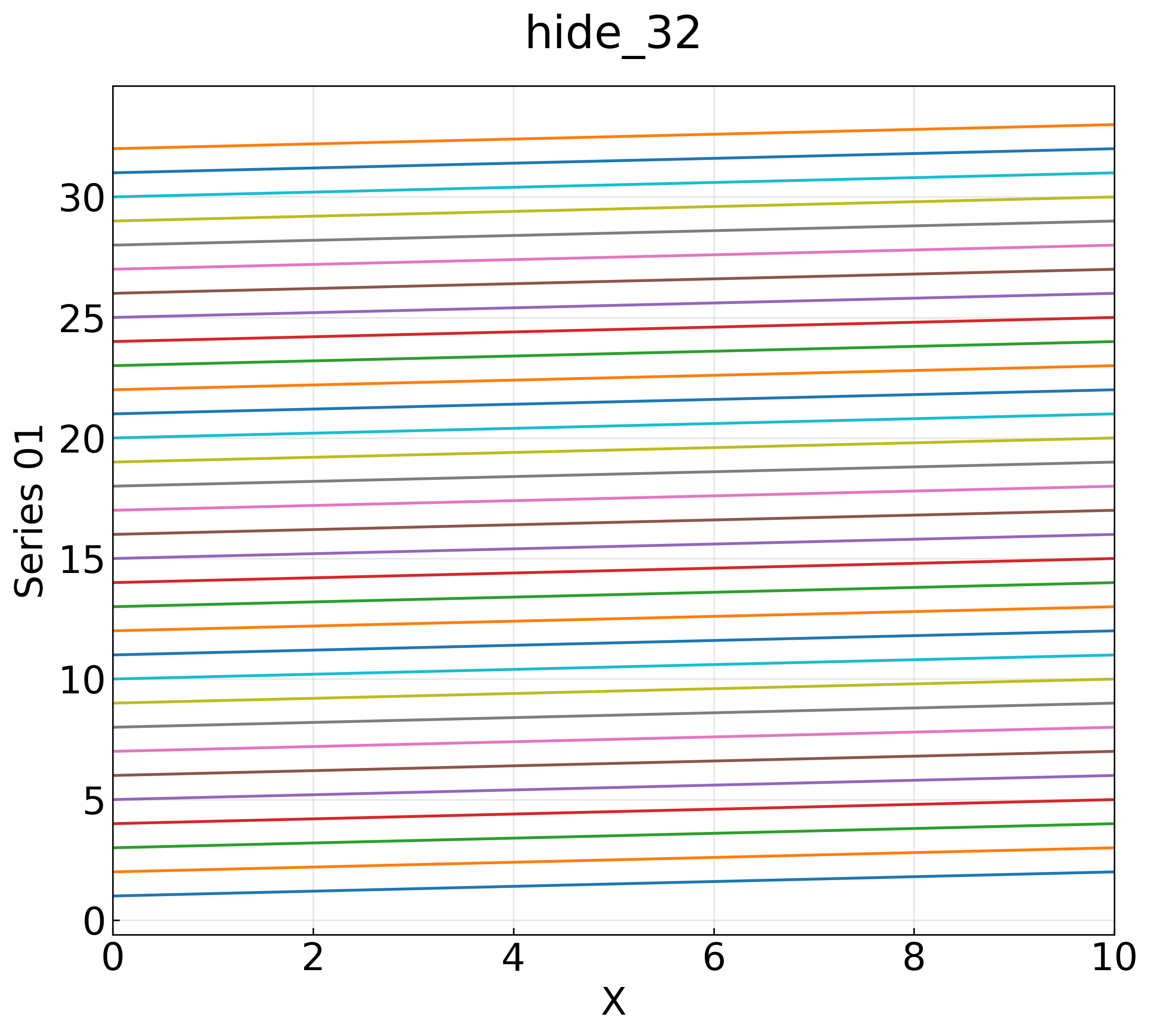
ケース6: 凡例を表示しない(hide / max_legend_items 超過)

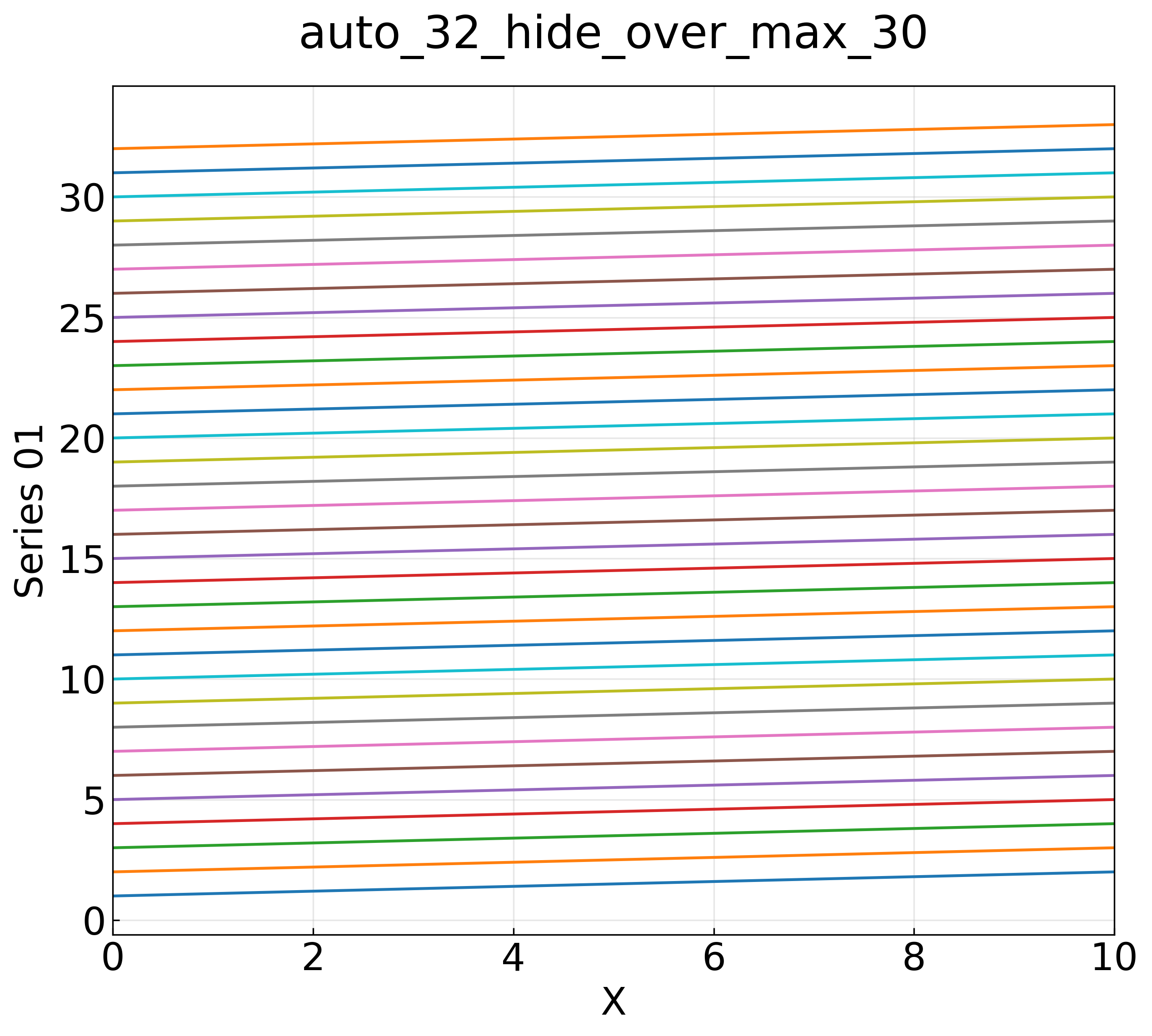
hide の明示指定と、max_legend_items=30 を32系列が超過して自動的に非表示になるケースです。出力画像は同等になります。
hide_32

auto_32_hide_over_max_30

 1
 2
 3
 4
 5
 6
 7
 8
 9
10
11
12
13
14
from pathlib import Path
from rdetoolkit.graph import csv2graph

if __name__ == "__main__":
    csv2graph(
        csv_path=Path("sample15/data.csv"),
        output_dir=Path("sample15"),
        x_col="x",
        no_individual=True,
        grid=True,
        title="hide_32",
        legend_policy="hide",
        max_legend_items=40,
    )
1
2
3
4
5
6
7
rdetoolkit csv2graph sample15/data.csv \
  --output-dir sample15 \
  --x-col x \
  --no-individual --grid \
  --title hide_32 \
  --legend-policy hide \
  --max-legend-items 40

オプションの説明

  • legend_bottom_threshold, --legend-bottom-threshold : auto が下側配置へ切り替える項目数のしきい値(デフォルト21。この値以上で切り替え)。Python では None、CLI では 0 以下を指定すると無効化できます。
  • legend_outside_threshold, --legend-outside-threshold : auto が右外側配置へ切り替えるしきい値(この値を超えたら切り替え)。デフォルト値(8 / 21)では「1〜8件 → inside、9〜20件 → outside_right、21件以上 → outside_bottom」となります。
  • legend_ncol, --legend-ncol : 下側配置の列数。項目数 ÷ 列数で段数が決まります(32項目 × 8列 = 4段)。
  • 外側配置ではプロット領域を維持したままキャンバスが拡張されるため、系列数が多くてもグラフ本体は潰れません。